H2Obudgt is a visual, GIS-based program for estimating past, present, and future water use in different parts of the State of Utah. It uses historical land use data as well as temperature and precipitation data to calculate water use. The output from this program includes estimated land use, evapotranspiration, and actual crop water demand for each year from 1970 to 2050. These estimates are given in three tables and are displayed graphically for visual interpretation.
 
 

Land Use Data: The Utah State Division of Water Resources has been collecting land use data within the state since 1985. This data has been collected through the use of aerial photography combined with field surveys to determine crop types. This data has been collected by major hydrologic basins, at the rate of about 1 basin per year. Table 1 below shows the different basins and when they were surveyed for land use.

Table 1: Land Use Survey Dates

Figure 1. Select Portion of Sevier River Basin Land Use

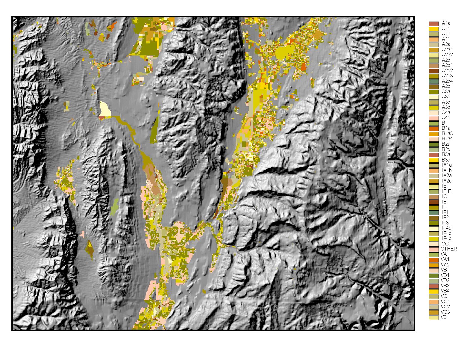
The original land use data is stored in ArcInfo polygon coverages, but the decision was made to have the H2Obudgt program work with gridded data. This means that the data must be converted to a grid format before running the program. The first reason for this decision is that gridded data is much faster to process. The second reason is that land use data in the near future is expected to be raster data from satellite imagery, rather than the laboriously digitized polygon data.

One limitation of this data that the user should be aware of is that the Division’s primary goal in collecting this data was to map agricultural water use. Therefore, natural water uses (riparian areas, forests, etc.) were not thoroughly mapped. Also, though an attempt was made to map urban areas, they were not given as much attention to detail as the agricultural lands.

Evapotranspiration Data: Dr. Robert Hill from Utah State University performed an extensive study of evapotranspiration rates across the State of Utah. The result of this study was the publication of average monthly evaporation rates for different plants in many representative agricultural sites throughout Utah. Included in this publication were monthly, crop-specific, Blainey-Criddle ET coefficients for each of the representative areas. Figure 2 below shows the locations of each of the sites.

One primary reason for using Dr. Hill’s data was that it has already been accepted for legal purposes by the State Engineer. This data is available from the Utah State Division of Water Rights web site at http://nrwrt1.nr.state.ut.us/manuals/consumpt/cfwea.htm

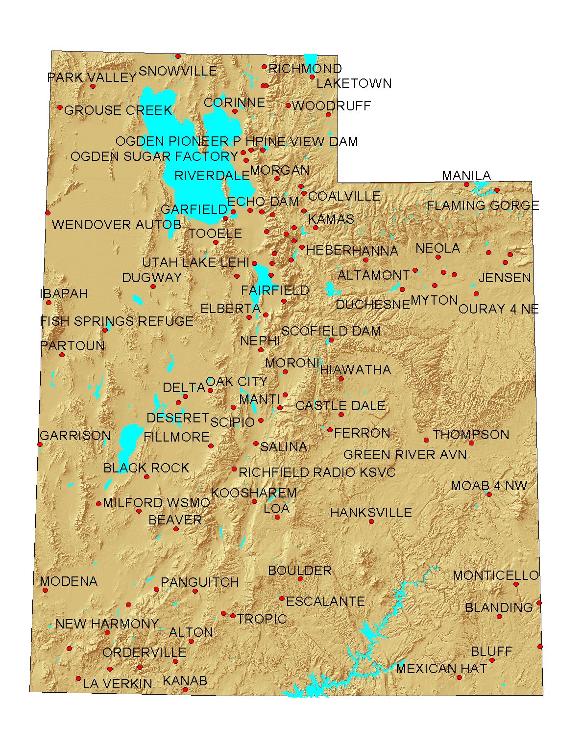
Weather Data: The weather data necessary for the H2Obudgt program includes monthly average min/max temperature and total monthly precipitation. Figure 3 below shows the stations in and around Utah for which data is readily available.

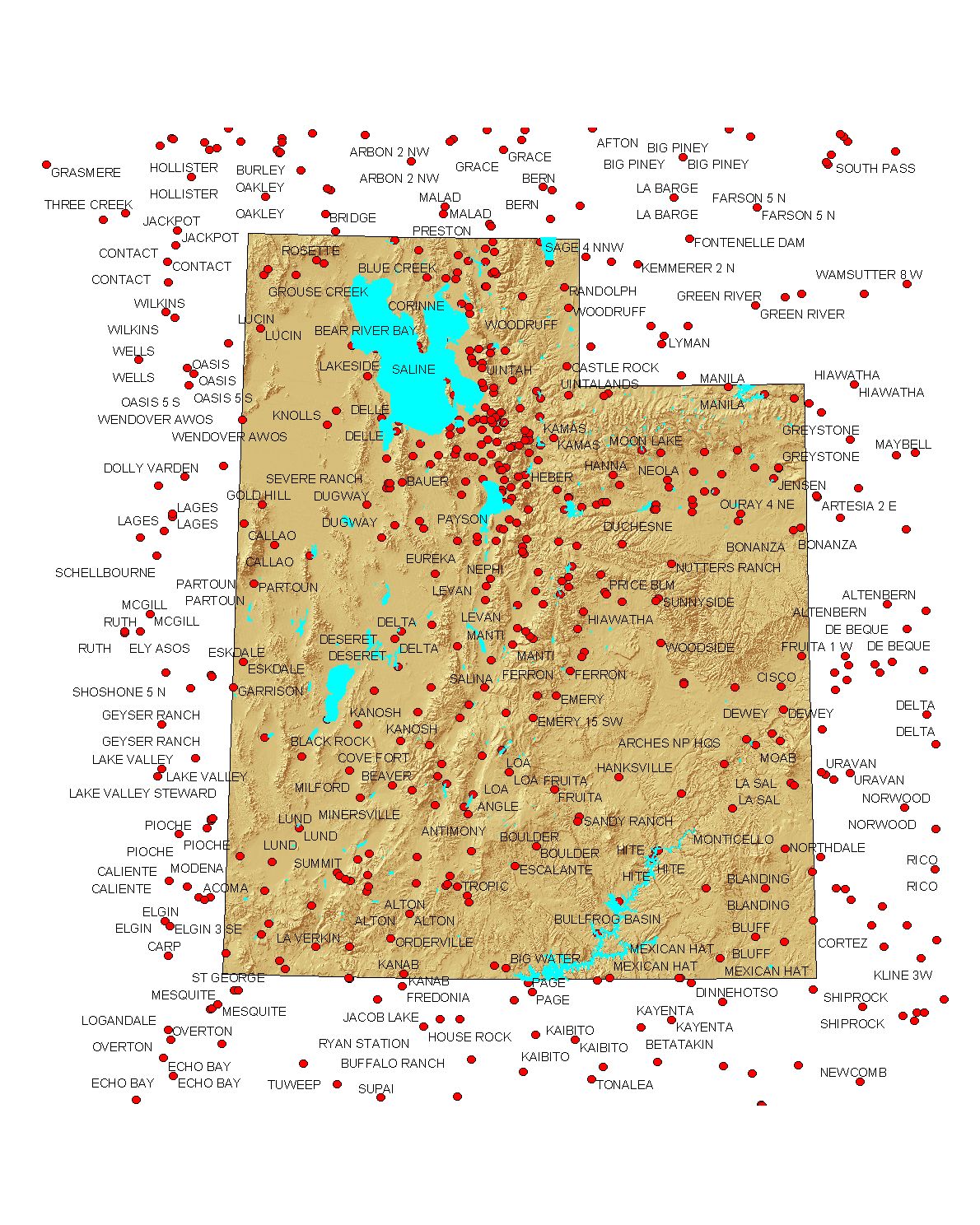
This weather data is available from the Utah Climate Center for all National Weather Stations in Utah at http://climate.usu.edu/weather/dataserv.htm

Elevation Data: Elevations of land use data were necessary in order to properly distribute weather data from stations at higher and lower elevations. A 90 meter digital elevation model (DEM) was stitched together from USGS data available at http://edcwww.cr.usgs.gov/doc/edchome/ndcdb/ndcdb.html
 
 

Land use trends: In a few basins, the Division of Water Resources has two separate years’ worth of land use data. Therefore, it is possible to analyze the trends in land use and interpolate between the two data points, as well as extrapolate for years outside of the two points. The data is linearly interpolated, and logical constraints (such as conservation of land area and non-negative land use values) are enforced to produce an estimate of the land use for each year between 1970 and 2050. This process is explained in more detail in the "Program Details" section of this report.

Evapotranspiration Estimation: In this program, the Blainey Criddle (BC) equation is used to calculate evapotranspiration. The BC equation is given below:

u = k_ck_t(tp/100) (1)

where u is the monthly consumptive use in inches, t is the mean monthly temperature in degrees Fahrenheit, p is the percentage of daylight hours of the year occurring during a particular month, k_c is a monthly growth stage coefficient, and k_t is a climatic coefficient that is computed as follows:

k_t = 0.0173t – 0.314, subject to k_t > 0.30 (2)

Soil Water Accounting: Two parameters are used to define the effect of rain on the water budget: a rainfall efficiency factor and the soil water holding capacity. The rainfall efficiency factor attempts to quantify the percent of rainfall that the plant can actually use. The remaining portion of the rain is assumed to evaporate before the plant can use it. The soil water holding capacity is important because the soil acts like a reservoir, storing up water during wet months for the plants to use in drier months. The soil water holding capacity is the depth of water that the soil is capable of storing and that a healthy plant can use without excess stress.
 
 

System Requirements: H2Obudgt requires ArcView 3.1 or higher, Spatial Analyst 1.1 or higher, S-PLUS 4.5 or higher, and S-PLUS for ArcView GIS 1.1. At least 64 megabytes of RAM are necessary in order to run the program, though more helps.

Setup: The following text files contain S-PLUS scripts that must be loaded into S-PLUS in order to run H2Obudgt:

• Bob Hill.txt
• Classify Land Use2.txt
• Potential ET Calculation.txt
• Weather Station3.txt

The H2Obudgt program was written in Avenue (ArcView’s programming language) and S-PLUS (a high-level statistical programming language). ArcView provides the primary user interface. There the user selects the study area, defines the land use data, and provides the necessary model parameters. Once all of the input data is provided and the program is started, all of the geographic analysis is performed in ArcView (through Avenue), while the main numeric calculations are performed in S-PLUS. The final output is presented in S-PLUS as well. Figure 4 shows a flowchart of the model execution.
 
 

Before beginning the program, the user needs to open a View window and add two gridded land use themes (with data from two different dates) and a polygon theme giving the boundaries of the study area. An example of the required data is shown below in Figure 5. The land use data is displayed on top of a relief map, and the black outline is a polygon theme defining the study boundaries.

Next, the user selects the "H2O budget" option from the WREtools drop-down menu. This brings up the dialog box shown in figure 6:
 
 

Now the user must fill in all the input boxes with appropriate values. Hitting the "Compute!!!!" button launches the main calculation routine.

Clip Land Use Data: The first thing the program does once it is started is clip the land use data according to the study boundary. It then calculates the total acreage of each type of land use listed in Table 2 for both years’ data.

Get Average Elevation: Next the program finds the average elevation of the surveyed lands by using the digital elevation model (DEM).

Find Closest Weather Stations: By using an incrementally increasing search radius, the program then locates at least 20 of the closest weather stations. The number 20 was arbitrarily deemed to be the smallest number of stations required to achieve a reliable regression of weather vs. elevation for the historical period between 1970-1997.

Find Closest ET Study Stations: Next ArcView uses the same method of incrementally increasing the search radius to find at least three of the closest ET study stations.
 
 

Write Text Files: ArcView then writes four text files to the project’s working directory. The first two files (luA*.txt and luB*.txt) contain the land use types and acreages found within the study area for the two different years. This data is written to files in the following format:

• A clipped land use grid theme
• A point theme of weather stations, with at least 20 of the closest stations selected
• A point theme of ET study stations, with at least 3 of the closest stations selected

Compute Land Use Trends: The first thing S-PLUS does once it has control of the program is read in the two land use files, luFN1 and luFN2, and compute land use trends. The trends are based on linear interpolation / extrapolation between the two years of data. However, two important logical constraints were placed on the extrapolations:

1. No land use category could have less than 0 acres
2. The total area of land use could not increase or decrease.

Reclassify Division Land Use Categories into ET Study Categories: The Division of Water Resources land use categories do not mesh exactly with the categories used in Dr. Hill’s ET study, so the following re-classification is performed in the program:

IA3a Alfalfa IA2b3 Beans

IA1e Orchard IA2a1 Corn

IA2a SP Grain IIA2b Other Hay

IIA2a Pasture IA1f Orchard

IA1a Orchard IA2b2 Garden

IA3d Pasture IA3b Other Hay

IA2b1 Potatoes IA2c Garden

IA2a2 Corn IA2b4 Garden

IA3c Turf IA2b Garden

IA1c Orchard IIB Other (No ET)

IIF4c E-Lake IIF3 E-Lake

IIF4 E-Lake IIF2 E-Lake

IIE E-Lake IIF4b E-Lake

IIF1 E-Lake IIF5 E-Lake

IIF4a E-Lake IIF E-Lake

IIC E-Lake IIA1b E-Lake

IIA1a E-Lake IIB-E E-Lake
 
 

Read in ET Study Data: The data from each of the ET stations listed in the bobFN file is read into S-PLUS. The important variables that are stored are:

1. Percent daylight for station – these are monthly values, so they are stored in a vector with 12 values.
2. "k" values for the Blainey-Criddle equation – there are 12 monthly k values for each crop type (15 crop types), so these are stored in a 12X15 matrix.
3. Average ET values – again, there are 12 average monthly ET values for each of 15 different kinds of crops, so these are stored in another 12X15 matrix.

Dr. Hill’s study tried to account for the major crops grown in each study area, but occasionally the Division of Water Resources mapped crops that were not listed for the region in the ET study. In this case, the crop coefficients were calculated as:

Read in Weather Data and Correct for Elevation: The weathFN file contains the names of all the weather stations to be used, and S-PLUS uses these names to retrieve the data associated with them. From this data, S-PLUS calculates the average monthly temperature for each month for each station as the mean of the maximum and minimum temperatures. Next, for each month it performs a robust, least-trimmed-squares regression of this temperature data vs. the elevation of the recording weather station. The month’s average temperature value is then approximated as the value of the regression at the average elevation of the land use. The precipitation is handled exactly the same way, except that precipitation is not given as max and min values that need to be averaged for each month.

The end results of this step are two 12 month X 81 year matrices (81 years from 1970 to 2050). One matrix contains average monthly temperatures and the other contains total monthly precipitation. The data from 1970 to the present extent of the data is historic data, while the data from then on is the average monthly data from the earlier data.

Calculate Monthly ET for each Crop Type: Next the temperature matrix is multiplied by the crop coefficient matrix and the percent daylight vector as given in the Blainey-Criddle equation (equations 1 & 2). This gives the crop water demand, or "potential ET" as the term is used in the Division of Water Resources.

Calculate Effective ET: After calculating the "potential ET", the program performs a water budget analysis by subtracting the amount of effective rainfall from the "potential ET". The rainfall is allowed to fill up the soil reservoir when it exceeds the crop water demand, and this soil water supply is then used in months with higher demand. The remaining water demand is what must be supplied from irrigation. This irrigation requirement is termed the "effective ET" by the Division of Water Resources.

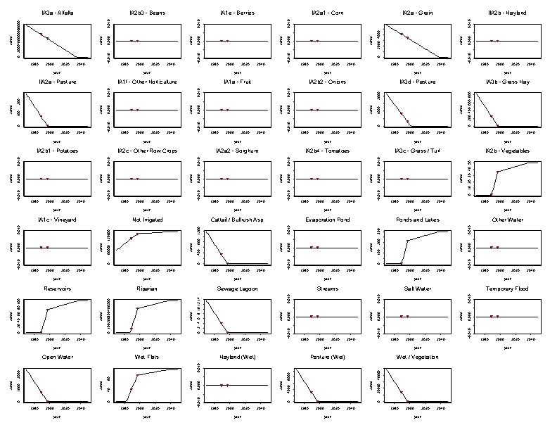
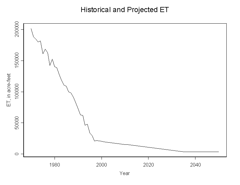
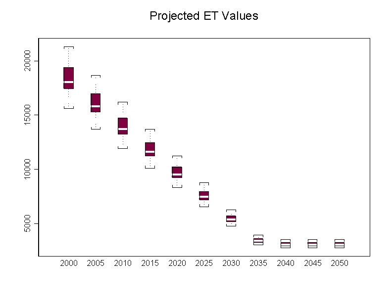
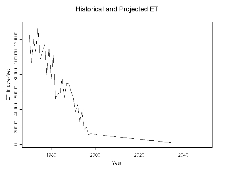
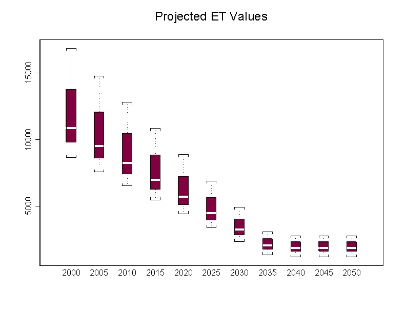
Plot Results: Finally, the results are visually plotted in S-PLUS. Figures 6-10 show results of a typical analysis.
 
 

Output Tabular Results: The final results are also presented in tabular form within S-PLUS, as shown in Figure 12. Three tables are produced:

• A table of acreages of different types of land use
• A table of yearly "potential ET" for each crop type and for each year from 1970 to 2050. This is the total amount of evaporated water, and is given in inches.
• A table of "effective ET", or the amount of irrigation required. A value is given for each crop type and for each year. Again, these values are reported in inches.

As of now, H2Obudgt is an unfinished program. There are still several components that need to be added. Right now the model ignores municipal and industrial (M&I) water use. A module to handle M&I water will hopefully be added in the coming months. The model also does not calculate reservoir evaporation, and this will need to be added as well. Finally, I would like to see records of water supply thrown into the budget calculations so that the model could produce an entire budget of supply as well as use.

Several existing features of the model need to be modified as well. This paper has already pointed out the ad-hoc methods of land use trend prediction and how these need to be more rigorously constrained. Another potential improvement in model performance may be gained by using monthly, gridded weather maps of the state produced by Dr. Donald Jensen. The use of this data would eliminate the need to regress against elevation, and could potentially provide a more reliable estimate of past weather.