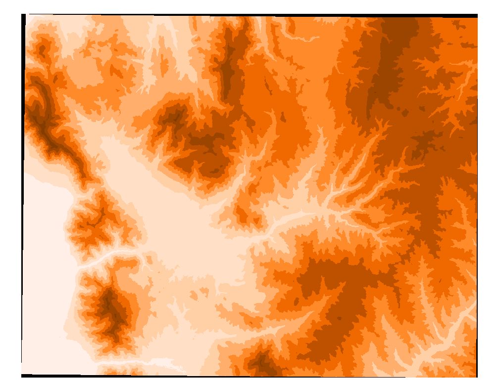
Figure 1. DEM of the research region
CONTENTS
INTRODUCTION
GOALS
APPROACHES OF
RESEARCH
DESCRIPTION
DATA
COLLECTION
DATA-PREPROCESS
WATERSHED
AND STREAM NETWORK DELINEATION
PRECIPITATION
RUNOFF
CONCLUSION
ONGOING
WORK
ACKNOWLEDGEMENT
Pineview Reservoir supplies drinking water for the city of Ogden, Utah. The reservoir is in the northwest of the Lower Weber Basin. In order to delineate source water protection areas, inventory significant contaminants in these areas, and determine the susceptibility of each public water supply to contamination, a Utah state government funded research project called source water protection assessment tools development takes this reservoir as the research object.
1.Delineate the watershed contributing to Pineview Reservoir;
2.Develop the relationship between mean annual runoff and mean annual precipitation, get the mean annual runoff for the whole watershed;
3.Estimate the total mean annual contaminant loads to the reservoir, focus on some specific constituents.
1.Download all the needed data from the Internet;
2.Two ways to get the mean annual precipitation data, first choice is to get it from PRISM, second choice is to use the weather stations data to develop the relationship between mean annual precipitation and elevation in this specific region, then use map calculator of ArcView to get the mean annual precipitation grid;
3.Use the gage stations data and the delineated sub-watersheds, get the mean annual runoff of each watershed contributing to the gage station; from the data groups ( precipitation, runoff ), use linear regression method to get the linear equation between mean annual runoff and mean annual precipitation, use this equation to get the whole mean annual runoff of this watershed;
4.Use the equation:
contaminant loads
= sum of Qi*Ci(Qi is mean annual runoff of each cell, Ci is the Event Mean
Concentration of specific constituents)
to get the mean
annual total contaminant loads.
1.DEM
I get the DEMs from USGS GEOSPATIAL DATABASE. I download the 7.5 minutes DEM, but some problem occurred when I deal with the North Ogden Quad. I cannot get the data using general method, so I asked Dr. Tarboton for help. He utilized MicroDEM to solve this problem. So I get the DEMs of the research region, altogether 15 Quads.
2.rf3
I get the river reach file from EPA BASIN2. I downloaded all the rf3 of the Lower Weber Basin.
3.Weather Station Data
From West US Weather Data, I download all the weather station data which is in or close to the Pineview Reservoir Watershed.
4.Gage Station Data
From EPA Stream DATABASE, I get the gage stations data, which is in the watershed.
5.Precipitation
From PRISM, I get the US WESTERN precipitation data.
1.DEM
After getting the raw DEMs, firstly I merge them. Then use Gapfill.exe(which is part of the software TARDEM ), fill the gaps in the DEMs.
Figure 1. DEM of the research region
2.rf3
Project the rf3 into Projection--UTM 1927,ZONE 12.
3.Weather Station data
After downloading the original data, I get the Excel
file-weathersta.txt, use comma delimited form to save it; then change the
suffix .txt to .cvs. In ArcVIEW, click Add event theme of view in
the menu bar, then choose weathersta.cvs, I create the point theme
weathersta.shp.
| station name | count number | lat (ddmm) | long (ddmm) | latitude | longitude | elevation (10ft) | elevation
(m) |
ann ppt(in) | start | end |
| HUNTSVILLE MONASTERY | 424135-5 |
4114 |
11143 |
41.233 |
-111.717 |
514 |
1567.7 |
22.79 |
11/1/76 |
12/31/98 |
| OGDEN PIONEER P H | 426404-3 |
4115 |
11157 |
41.250 |
-111.950 |
435 |
1326.75 |
20.82 |
1/1/02 |
12/31/98 |
| OGDEN SUGAR FACTORY | 426414-3 |
4114 |
11202 |
41.233 |
-112.033 |
428 |
1305.4 |
17.29 |
1/1/24 |
12/31/98 |
| PINE VIEW DAM | 426869-5 |
4115 |
11151 |
41.250 |
-111.850 |
494 |
1506.7 |
30.68 |
7/1/48 |
12/31/98 |
| RIVERDALE POWERHOUSE | 427318-3 |
4109 |
11200 |
41.150 |
-112.000 |
440 |
1342 |
18.4 |
1/1/28 |
2/28/91 |
| UINTAH | 428885-3 |
4109 |
11155 |
41.150 |
-111.917 |
483 |
1473.15 |
22.26 |
7/1/48 |
4/30/60 |
| WEBER BASIN PUMP PL 3 | 429346-3 |
4107 |
11155 |
41.117 |
-111.917 |
491 |
1497.55 |
25.7 |
5/2/62 |
12/31/98 |
| BRIGHAM CITY | 420924-3 |
4129 |
11202 |
41.483 |
-112.033 |
430 |
1311.5 |
19.41 |
7/2/48 |
5/31/74 |
| COALVILLE | 421588-5 |
4055 |
11124 |
40.917 |
-111.400 |
555 |
1692.75 |
16.11 |
7/1/48 |
12/31/98 |
| ECHO DAM | 422385-5 |
4058 |
11126 |
40.967 |
-111.433 |
547 |
1668.35 |
14.53 |
7/1/48 |
12/31/98 |
| FARMINGTON | 422721-3 |
4059 |
11154 |
40.983 |
-111.900 |
427 |
1302.35 |
19.28 |
7/1/48 |
5/31/65 |
| FARMINGTON WHSE STN | 422726-3 |
4059 |
11153 |
40.983 |
-111.883 |
433 |
1320.65 |
22.92 |
7/1/48 |
12/31/98 |
| MORGAN | 425826-5 |
4103 |
11141 |
41.050 |
-111.683 |
507 |
1546.35 |
18.27 |
7/1/48 |
12/31/98 |
Table 1. Weather Station information
4.Gage Station data
After downloading the original data, I get the Excel
file-gagesta.txt, use comma delimited form to save it; then change the file name
to gagesta.cvs. In ArcView ,click Add event theme of view in the
menu bar, then choose gagesta.cvs, I create the theme gagesta.shp.
|
|
|
|
|
|
|
|
|
|
|
|
|
|
|
|
|
|
|
|
|
|
|
|
|
|
|
|
|
|
|
|
|
|
|
|
|
|
|
|
|
|
|
|
|
|
|
|
|
|
|
|
|
|
|
|
|
|
|
|
|
|
|
|
|
|
|
|
|
|
|
|
|
|
|
|
|
|
| |
|
|
|
|
|
|
|
|
|
|
|
|
|
|
|
|
|
|
|
|
|
|
|
|
|
|
|
|
|
|
Table 2. Gage Station information
5.Precipitation
I use two approaches to get the precipitation data. The method of using elevation v.s. precipitation will be introduced at the latter part. Here I will introduce the PRISM data. When I tried to get the PRISM data before the oral presentation, I failed to enter the data download page. But several days ago, when I tried to work on it again, I succeeded. This is funny.
There are two choices to get the PRISM data, one to get the raster data, another to get the vector shape file. I tried two methods, and I found the raster ASCII data can get a higher resolution, so I use the former method. But there is a big problem, because the ASCII data format cannot be projected in ArcView, then I worked out a solution for it. First I save it as ASCII file, then from file menu, click the import data source, choose ASCII raster, get the grid utahppt. The PRISM data grid is in geographic coordinates, in order to project it, first I convert it to shape file, name it utahppt.shp. Then I project the shape file utahppt.shp into UTM-1927, ZONE 12. Then I convert it back to grid, save it as ogdenppt. Now the precipitation grid is in the same projection as other themes.Then use clip features to get the relevant grid for my research region.
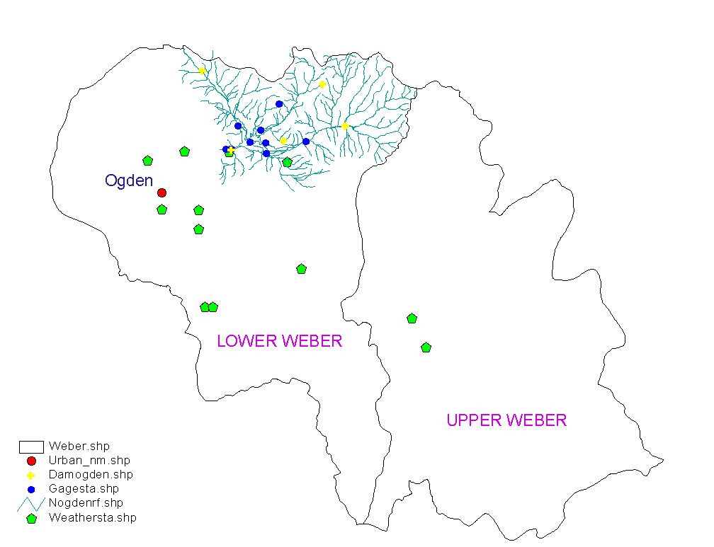
Figure 2.Gage Stations, Weather Stations, rf3 in the
watershed
Watershed and Stream Network Delineation
I use the CRWR-PrePro to delineate the watersheds and stream
network for the Pineview Reservoir Watershed. Following are the
procedures:
1.burn DEMs;
2.fill sinks;
3.flow directions;
4.flow accumulation;
5.flow
outlets;
6.add outlets; (I add all the gage stations as
outlets, most of the points are not on the streams, so I change their positions
to the nearest point on the streams.)
7.subwatershed
and stream network delineation;
8.vectorize the
subwatersheds and streams;
9.merge all the
subwatersheds on the upstream of the gage stations;
10.create shape files for all the subwatersheds which contributes to the
gage stations;
11.create mask grid for the Pineview
Reservoir Watershed and mask grids for all other subwatersheds;
12.use the map calculator and the mask grid, get the DEM for the
Pineview Reservoir Watershed. 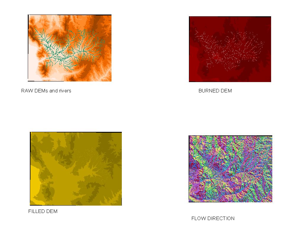
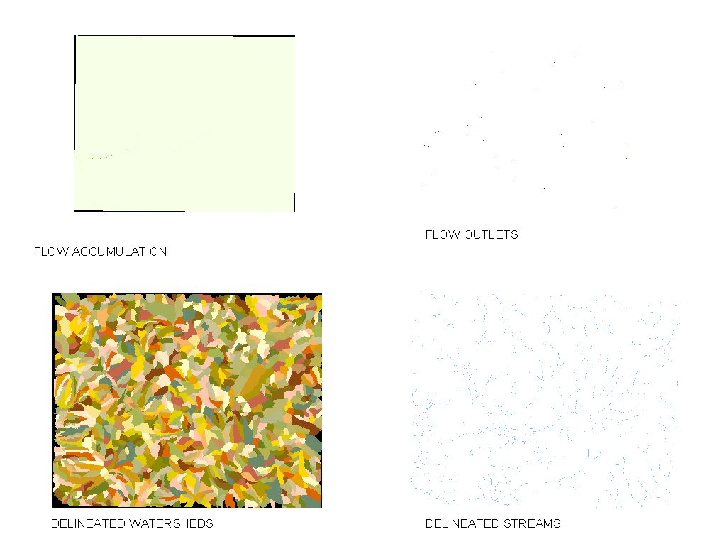
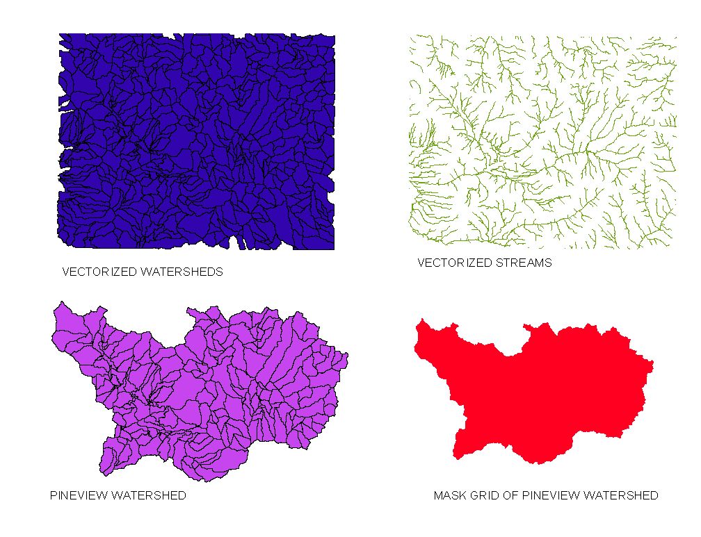
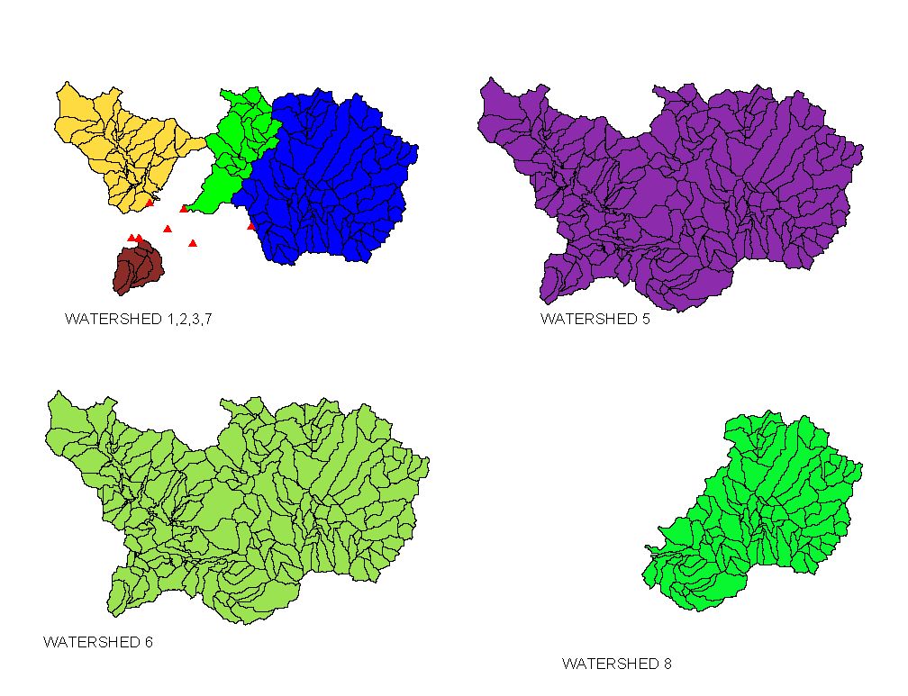
Figure 3 CRWR-PrePro
PRECIPITATION
I use two methods to
get the precipitation grid.
1.Use the weather station
data, then use Excel's linear regression method to develop the
relationship between elevation and mean annual precipition.Because this is a
small watershed, and the horizontal geographic environment is almost the
same,but the vertical elements, i.e., the elevation varies greatly. So we can
conclude that in this region, the main element influences the climate(including
precipitation ) is elevation. And the comparison with PRISM data shows this
conclusion is correct.
| station name | count number | lat ddmm | long ddmm | latitude | longitude | elevation 10ft | ele-m | ann ppt(in) | start | end |
| HUNTSVILLE MONASTERY | 424135-5 |
4114 |
11143 |
41.23333 |
-111.717 |
514 |
1567.7 |
22.79 |
11/1/76 |
12/31/98 |
| OGDEN PIONEER P H | 426404-3 |
4115 |
11157 |
41.25 |
-111.95 |
435 |
1326.75 |
20.82 |
1/1/02 |
12/31/98 |
| OGDEN SUGAR FACTORY | 426414-3 |
4114 |
11202 |
41.23333 |
-112.033 |
428 |
1305.4 |
17.29 |
1/1/24 |
12/31/98 |
| PINE VIEW DAM | 426869-5 |
4115 |
11151 |
41.25 |
-111.85 |
494 |
1506.7 |
30.68 |
7/1/48 |
12/31/98 |
| RIVERDALE POWERHOUSE | 427318-3 |
4109 |
11200 |
41.15 |
-112 |
440 |
1342 |
18.4 |
1/1/28 |
2/28/91 |
| UINTAH | 428885-3 |
4109 |
11155 |
41.15 |
-111.917 |
483 |
1473.15 |
22.26 |
7/1/48 |
4/30/60 |
| WEBER BASIN PUMP PL 3 | 429346-3 |
4107 |
11155 |
41.11667 |
-111.917 |
491 |
1497.55 |
25.7 |
5/2/62 |
12/31/98 |
| BRIGHAM CITY | 420924-3 |
4129 |
11202 |
41.48333 |
-112.033 |
430 |
1311.5 |
19.41 |
7/2/48 |
5/31/74 |
| COALVILLE | 421588-5 |
4055 |
11124 |
40.91667 |
-111.4 |
555 |
1692.75 |
16.11 |
7/1/48 |
12/31/98 |
| ECHO DAM | 422385-5 |
4058 |
11126 |
40.96667 |
-111.433 |
547 |
1668.35 |
14.53 |
7/1/48 |
12/31/98 |
| FARMINGTON | 422721-3 |
4059 |
11154 |
40.98333 |
-111.9 |
427 |
1302.35 |
19.28 |
7/1/48 |
5/31/65 |
| FARMINGTON WHSE STN | 422726-3 |
4059 |
11153 |
40.98333 |
-111.883 |
433 |
1320.65 |
22.92 |
7/1/48 |
12/31/98 |
| MORGAN | 425826-5 |
4103 |
11141 |
41.05 |
-111.683 |
507 |
1546.35 |
18.27 |
7/1/48 |
12/31/98 |
Table 3 Weather Station Data
Graph 1 Equation between ELEVATION and PRECIPITATION
Here I get the equation P=0.7239*ELE-495.28, where P stands for precipitation(mm), and ELE is elevation(m). Now I use the map calculator to make computation for DEMs of the watershed, so I get the precipitation grid for the watershed.
After this, I make mask grids for each sub-watershed, i.e.,1,2,3,5,6,7,8,then use these masks to get the precipitation grids for each sub-watershed.
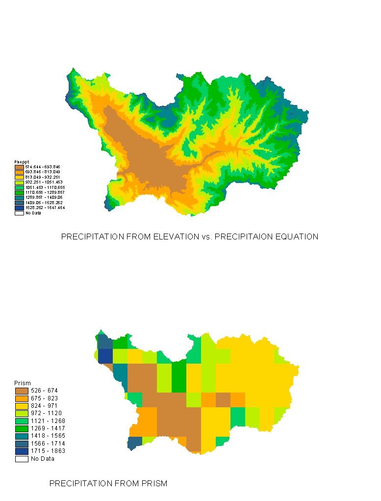
Figure 4.Precipitation from two approaches
2.Get the PRISM data for the whole UTAH state, then clip it to show only the part for the research region. This is shown above.
From the Legend/Statistics, I get the mean annual precipitation from method 1 is 990mm, from method 2 is 926mm. The difference is (990-926)/926*100%=6.91%. This difference is small, and the distribution of the precipitation resembles each other, so we can make a conclusion the method 1 is reliable. And furthermore, the precipitation from method1 has a 100 times higher resolution than from PRISM, cause in PRISM, the cell size is 3000m, while in method 1,the cell size is the same as the DEMs, which is 30 meters.
From the precipitation grids for each sub-watershed, I get the mean precipitation for each sub-watershed, i.e., mean precipitation for each gage stations.
From the gage station data, I get the mean runoff for each gage
station. Using the following equation: Mean runoff = mean annual stream flow
/(drainage area).Then use the mean precipitation data for each gage station
to form data groups. Use Excel again, to develop the linear equation for these
two terms.
| SUBWATERSHED id | mean precipitation(mm) | mean runoff (mm) |
|
1 |
933.77 |
170 |
|
2 |
1079.21 |
185 |
|
3 |
1095.34 |
288 |
|
5 |
989.93 |
88 |
|
6 |
989.55 |
108 |
|
7 |
959.02 |
304 |
|
8 |
1036.07 |
136 |
Table 4.Mean annual precipitation vs.Mean
annual runoff for the gage stations
Graph 2.Equation for mean annual runoff vs. mean annual precipitation
Now use the equation R=0.2796*P-100.21, (where R stands for mean annual runoff (mm), P is mean annual precipitation (mm) ), we can use map calculator to get the mean annual runoff for the whole watershed.
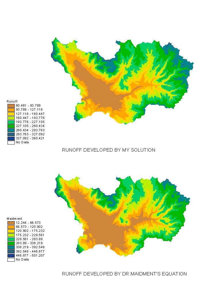
Figure 5.Runoff for the watershed from two different
approaches
I checked my solution with Dr. David Maidment's approach, which is
R = 0.51*P - 339 ,for P >= 800mm and R = 0.00064* P * exp(0.0061* P) ,for P < 800 mm.
From this, I also get the runoff grid for this watershed. The two solutions are shown as above, we can see that the runoff value and its distribution is very alike. The mean runoff for this region is 176mm, from my solution, and it's 171mm, from Dr.Maidment's approach. The difference between these two value is (176-171)/176*100% = 2.8%,which is trivial. Though this kind of relationship may be restricted in every specific region, we can also get an approximate value for the regions with almost the same geographic background. And from this, I can conclude that this solution is effective enough, so I can use it for further work.
After this, I will try to get the LULC (LAND USE AND LAND COVER DATA) , and investigate the Point and Non-Point contamination sources in this region. Then try to get the EMC (event mean concentration) for some specific constituents, use the equation TOTAL CONTAMINANT LOADS = SUM OF (EMC*RUNOFF) to get the mean annual total contaminant loads to the Pineview Reservoir. Then use this information to do some assessment for the contamination in this region, and make technological suggestions for taking some relevant measurements.
ACKNOWLEDGEMENT
I must thank Dr.Tarboton for his instruction and especially for his help to
get the DEM data. Otherwise, I can not finish this term paper. And I also must
thank my classmates for their help.