EVALUATION OF PRECIPITATION THRESHOLDS FOR
GROUND SATURATION & SLOPE STABILITY
By, Erkan Istanbulluoglu
Utah State University
Civil & Environmental Engineering Dept.
84322-4110, Logan UT
INTRODUCTION
Topography plays an important role in the hydrologic response
of a catchment to rainfall. For example, topography can affect the location of
zones of surface saturation and the distribution of the soil water (i.e., the
soil water content overlying an impermeable or semiimpermeable soil horizon at
shallow depth). The likelihood of soils becoming saturated increases at the base
of slopes and in depressions or swales where there is convergence of both
surface and subsurface flow (Barling et al., 1994). The spatial distribution of
soil water is a very important issue to estimate the subsurface and surface flow
and evaluate the sediment production and transport processes within a
watershed.
With the development of digital terrain models, capable of
analyzing large sets of digital elevations, it is now possible both to quantify
the detailed topography of landscapes and to explore process based models in
explaining mappable features (Dietrich et al., 1993). Terrain-based indices have
been developed predicting the spatial distribution of soil water content and the
location and size of zones of surface saturation under an assumption of
steady-state flow [eg., Beven and Kirby, 1977, 1979 and O'Loughlin, 1986].
Derivation of these indices which simply represent the key factors like
topography in physical processes has encouraged the derivation of saturation,
erosion and slope stability thresholds [eg., Dietrich et al., 1993].
This study aims to evaluate the threshold rainfall depths
required for ground saturation, slope stability and runoff and to construct a
functional relationship between rainfall and spatial probability of those
variable within a watershed.
THE STUDY AREA
Site Description
The study area is in the Silver Creek drainage, a tributary to the Middle
Fork of the Payette River in southwestern Idaho. Coordinates of the center of
the project area are approximately 44o25’N latitude, and
115o45’W longitude.
Annual precipitation on the study
area averages about 890 mm with most occurring during the winter months. Summers
are hot and dry with occasional, localized convective storms. More generalized
frontal types of rains are common in May and June and in the fall in late
September and October. About 65% of the annual precipitation is as snow that
produces an average maximum snow melt water equivalent of about 55cm.
Soils are weakly developed with an A horizon ranging from 5 to 25 cm thick
and overlying moderately weathered granitic parent material. Soil textures are
loamy sands to sandy loams and depth to the bedrock is usually less than 100 cm.
Shallow soils less than 20 cm deep are common on ridges and south slopes.
Hillslopes in the area are steep, ranging from 15 to 40 degrees, and are
highly dissected. Vegetation varies in response to change in slope aspect and
and soil properties and is characterized by principal vegetation habitat types,
which are Douglas-fir/white spirea and Douglas-fir/nineninebark, both in
ponderosa pine phase ( Megehan et al., 1991).
Data Preparation for GIS/Arc-View
Digital elevation model (DEM) of Silver Creek is required for the study.
There are two DEM data sources (that I know) from which one can do data
downloading. They are;
*US Geographical Survey (USGS); http://mcmcweb.er.usgs.gov/status/dem_stat.html
*GIS Data Depot ; http://www.gisdatadepot.com/
I used the USGS page and downloaded 4 quads where the Silver Creek should be
located. It is sometimes hard to figure out the exact location that one wants to
download in USGS DEM. Digital Raster Graphics (DRG) may assist one to find out
the location of the region he or she is working. DRG of the region downloaded
from GIS Data Depot for the study.
 The downloaded data was
imported to Arc-View, merged and gapfilled. TARDEM was used to calculate the
flow directions with D infinity approach and specific catchment area
(contributing area per unit contour length). The Dinf approach assigns a flow
direction based on steepest slope on a triangular facet (Tarboton, 1997). The
approach is depicted below.
The downloaded data was
imported to Arc-View, merged and gapfilled. TARDEM was used to calculate the
flow directions with D infinity approach and specific catchment area
(contributing area per unit contour length). The Dinf approach assigns a flow
direction based on steepest slope on a triangular facet (Tarboton, 1997). The
approach is depicted below.
Figure 1. Flow direction defined as steepest downward slope on planar
triangular facets on a block centered grid.
Slope of each grid cell was calculated by SINMAP (Pack et al., 1998), which
is a software for terrain stability mapping. Channel network was delineated
using upwards curved grid cells method one of the channel network delineation
options available in TARDEM. DEM of the Silver Creek which is 25.5
km2, with contours of 40 m interval and delineated channel network is
given below. (Cell size is 30mx30m)
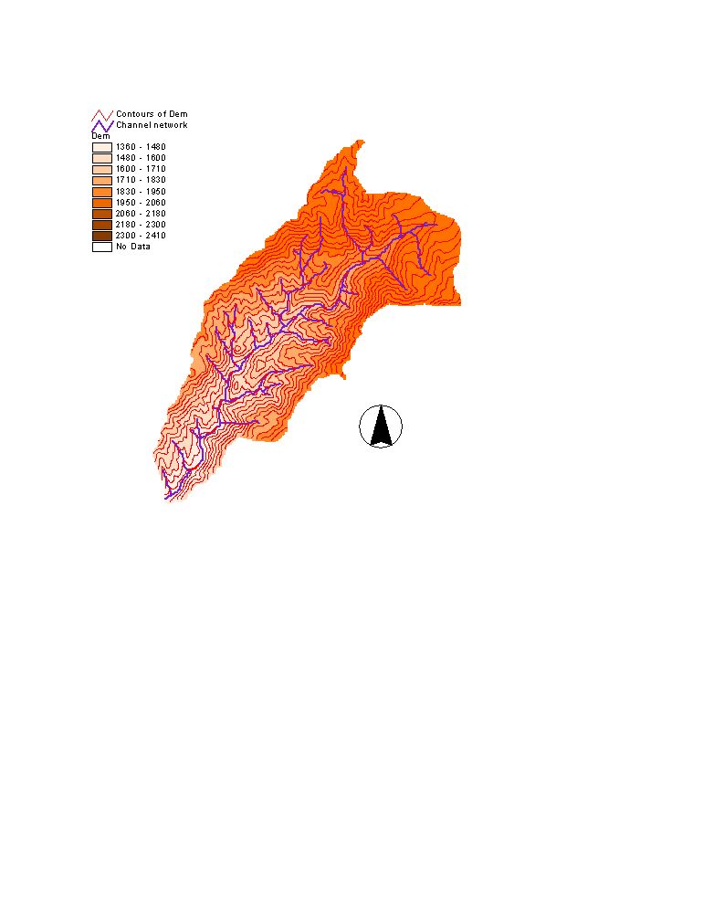
Figure 2. DEM of Silver Creek its channel network and contours
of 40 m interval 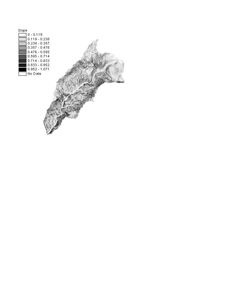
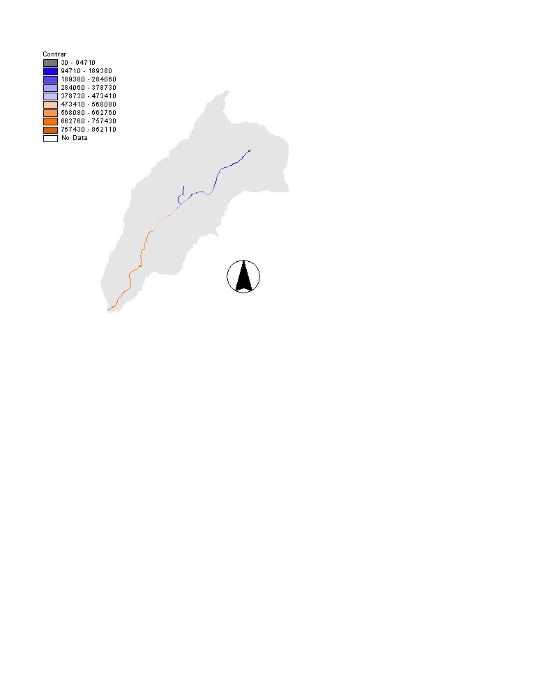
Figure 3. Slope and contributing areas per unit contour length of Silver
Creek
Slope and contributing area per unit contour length of Silver Creek is
presented above.
THEORETICAL CONSIDERATIONS
Groundwater
Sediment production due to landsliding and erosion, and
sediment transport in hillslopes deal with the ground saturation, so that
understanding the groundwater behavior is a key term to better evaluate the
hillslope processes.
Beven (1981) concluded that models models based on kinematic
wave formulation may be better than those based on the extended
Dupuit-Forchheimer assumptions for predicting water table profiles and
subsurface flow hydrographs. Assuming the subsurface flow is parallel to the
ground surface in a thin soil mantle, steady-stead subsurface flow can be in a
form of kinematic wave approximation as;
 (1)
(1)
where qi is the discharge per unit contour length at
a point (i) in the catchment (L2/T), K is the saturated
hydraulic conductivity (L/T), hwi is the subsurface water depth (L)
perpendicular to the slope and q is the slope angle (Wu
and Sidle, 1995). When a lateral water flux occurs during periods of
precipitation, the soil water content increases systematically in the downslope
direction. Topographic divergence and convergence also also affects the lateral
movement of water and the soil water content. The water table can be represented
as the result of steady average vertical recharge rate R, (L/T), so that any
point i on a catchment with a specific catchment area of ai
subsurface flow would be (Barling et al., 1994)
 (2)
(2)
Dietrich et al., (1992) claim that, for steady state shallow subsurface flow,
R term in the equation above can be considered as "precipitation - evaporation -
deep drainage", but in this study R is called shortly precipitation. Depth of
water table at a point i in the catchment can be estimated by combining (1) and
(2) and solving for hwi;
 hwi=h (3)
where h is the soil tickness perpendicular to slope. At any point where
hwi exceeds h, the ground will be saturated and any amount of
precipitation will cause runoff (Qi) at that point as,
 (4)
(4)
in the equation Khi can be written as Ti which is the
transmissivity in (L2/T). Due to differences in the specific
catchment area from which the subsurface water drains, the rainfall amount to
saturate the ground would be spatially distributed in a watershed. At a point i,
precipitation amount required for ground saturation can be estimated by setting
Qi to 0 and solving for Ri which will be,
 (5)
(5)
any precipitation rate greater than that Ri will produce runoff at
that point.
The steady state assumption implies that the specific upslope
area is an appropriate surrogate for the subsurface flow rate. This is only true
if recharge rate to a perched water table occurs at a constant rate for the
length of time required for every point on a catchment to reach subsurface
drainage equilibrium. In most cases, the velocity of the subsurface flow is so
small that most point on a catchment only receive contributions from a small
portion of their total upslope contributing area and the subsurface flow regime
is in a state of dynamic nonequilibrium (Barling et al., 1994). Interstitial
velocity of subsurface flow may be calculated as proposed by Barling et al.,
(1994)
 (6)
(6)
where v is the interstitial velocity of subsurface flow and
h is the effective porosity. In the equation above it
may be more accurate to use sinq rather than tanq. The total length of time required to observe a
steady-state subsurface flow at a point i on the catchment which has a
contributing area per unit contour length of ai may be calculated
as;
 (7)
(7)
in the equation ti may be evaluated as the time of
water input to the perched water in the contributing area of that point. This
water input time can be rainfall duration + drainage time + snow melting period
or which one is present in the watershed. For any time t when t
<ti contributing area per unit contour length would be (a(t)) but,
a(t)<ai. This concept requires us to rewrite the ai
terms in equations (2),(3) and (4) when t <ti.
When evaluating long term periods for example at a mountainous watershed which
receives plenty of snow, in the snowmelt period most of the watershed can be
assumed to reach to equilibrium and producing steady-state subsurface flow.
However this concept may be very important while evaluating the affects seasonal
precipitation to slope stability, landsliding and erosion.
Slope stability
The infinite slope stability model factor of safety (ratio of
stabilizing to destabilizing forces) can be written as below (Pack et al.,
1998).
 (8)
(8)
In the equation above FS is the factor of safety between 0 and
1, C is the combined cohesion, w the relative wetness, r the water to soil
density ratio, and f is the internal friction angle. C,
w and r can be defined as;
 (9)
(9)
 (10)
(10)
 (11)
(11)
In the equations; Cr and Cs are root and
soil cohesion [N/m2], rw and
rs are water and soil density
[kg/m3], and g is the gravity of acceleration [9.81 m/s2].
When FS<1 at a point, a lndsliding may occur.
Threshold theory for slope instability was given by Dietrich et
al.,(1992) which is,
 (12)
(12)
where, a/b is the area per unit contour length and S is slope.
Slope instability occurs where a/b equals or exceeds the term on the right-hand
side. In the equation R is constant for the whole watershed. In this study to
explore the spatial variability of R causing FS≤1, another form of threshold
relation is proposed by equating FS to 1 in (8) and solving for R in (10), which
is simply,
 (13)
(13)
While using the above equation only ai and q are considered as spatially distributed and the other
parameters are lumped. However in the watershed where reliable measurements are
available T, C and f can be used as spatially
distributed parameters. Using (13) one can calculate the rainfall rates required
to cause FS≤1 at any point of the watershed if that point is capable of
generating FS≤1 due to R. Because there would be points in the watershed even
saturated but still stabile (FS>1) because of the dominant affects of other
parameters associated with FS.
RESULTS & DISCUSSION
In the analyzes of ground saturation and slope stability
in Silver Creek the soil parameters are lumped in the watershed. The
lumping of similar parameters was done by Barling et al.,(1994); Dietrich
et.al.,(1992); Dietrich et.al.,(1993) and Wu and Sidle (1995) due to the lack of
reliable amount of measured values. Those parameters are saturated hydraulic
conductivity (K=0.833m/h), soil depth (h=0.6m), effective porosity (h =0.4), internal friction angle (f=30) and combined cohesion (C=0-0.2) are lumped in the
watershed referring to previous studies by Megehan et.al,(1991); Gray and
Megehan (1981). In combined cohesion two values are assumed. In the referred
paper the cohesion was measured as 0, however a cohesion of 0.2 is also taken
into because of possible changes in C in time due to forest fires and
removal.
Time of Equilibrium
In order to evaluate the time required to reach steady-state conditions in
the watershed,
interstitial velocity of subsurface flow in each grid cell
was calculated by(6) in m/h.
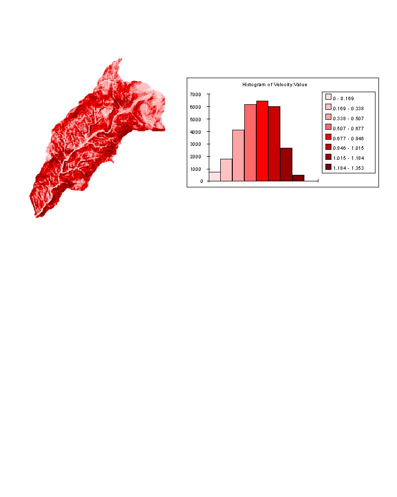
Figure 4.Interstitial velocity
distribution for each grid cell
The velocities range between 0 at grids with no slope and 1.353
m/h at the steepest slopes. Time required to reach an equilibrium in most of the
watershed (83%) is estimated as 30days. In this 30 day time subsurface flow
should receive either precipitation or snowmelt. The grid cells which come to an
equilibrium (7.7% of the watershed) after 2 days of recharge are below, colored
in red . The length of grid cells are 30m, in the ones which have an
interstitial velocity less than 30/2, 15 m/day the water starts to travel from
one end doesn't reach the other end. They are colored in gray in the map.
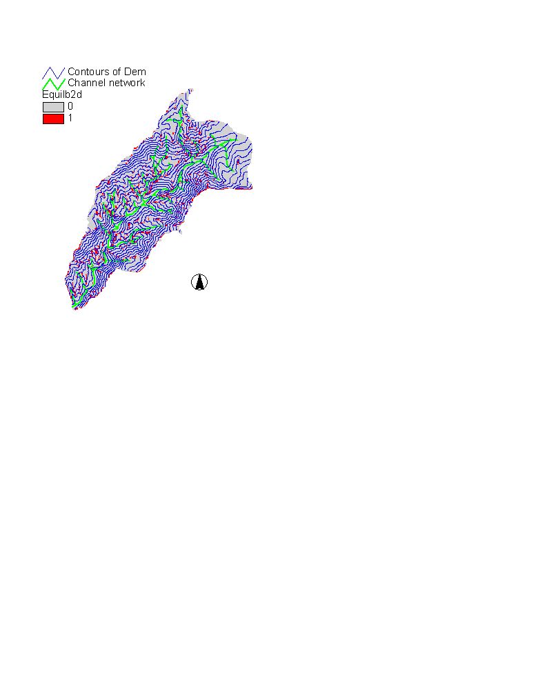
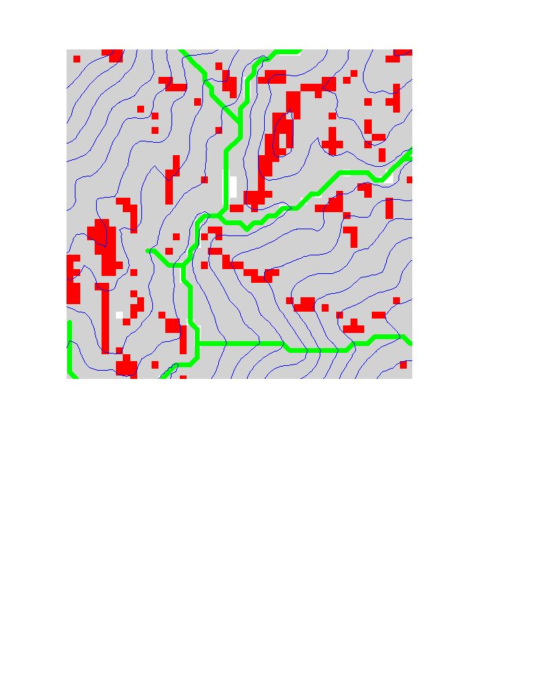
Figure 4. Grid cells in equilibrium after 2 days of continuos
recharge
The same picture after 30 days of continuos recharge is,
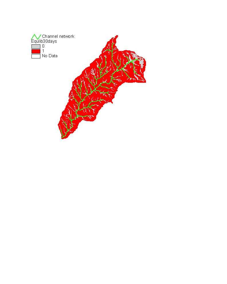
Figure 4. Grid cells in equilibrium after 30 days of continuos
recharge
As it can be seen from Fig. 4. The watershed comes to almost
steady state subsurface flow condition. This concept has a vital importance
especially in the watershed which has shallow soils with high infiltration
capacity. Because in those watersheds the source of runoff is due to saturation
below mechanism and after reechoing steady-state condition saturation would be
achieved in downslope regions and sediment production and transport may increase
due to erosion and landsliding.
Saturation
Watershed saturation under steady state recharge and subsurface was evaluated
by eqn.(5). The areas with steep slopes and small contributing area would
require more precipitation to get saturated. Even those areas require a lot more
precipitation they may come to steady state condition in a couple of days as
shown in Fig.2. Areas located close to the channel network and those of which
have a large contributing area can be saturated with very low intensities of
precipitation rate (recharge). However this constant precipitation rate should
last very long time in order to reach the steady-state conditions.
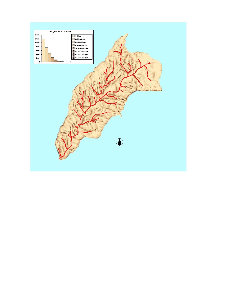
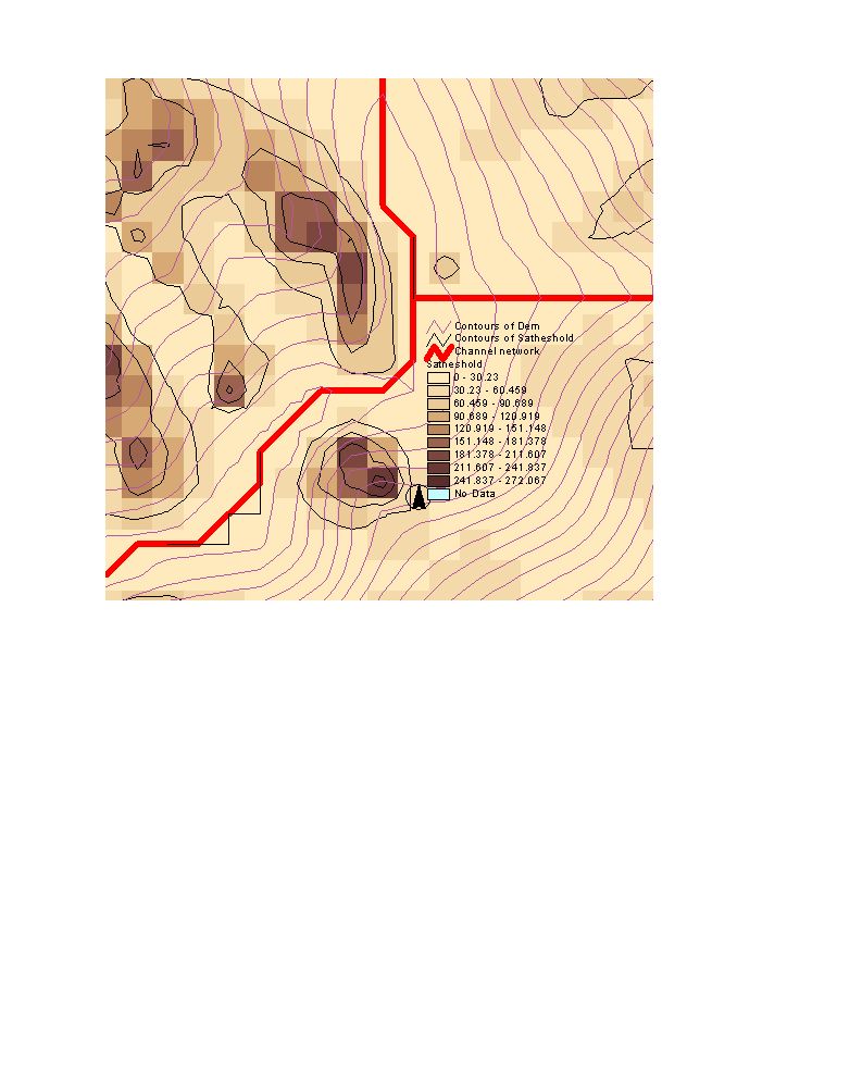
Figure 5. Precipitation rates required for saturation, (precipitation rates
are in mm/day. (a) precipitation rates for the entire watershed (b) the selected
region with 10 m contour interval of DEM and 50 mm/day contour interval of
saturation precipitation)
This saturation information may be useful for practical
calculation purposes for erosion and sediment transport. Because runoff is very
important for either erosion or sediment transport. In a watershed where the
steady-state precipitation thresholds for saturation are known and plotted at a
graph as precipitation rate on X axis and watershed saturated area in (%) on Y
axis, one can estimate the runoff for a given precipitation rate and portion of
the watershed contributing to runoff.
Slope stability
Before calculating the slope stability threshold precipitation required for
each cell, distribution of FS over the entire watershed under a best and a worst
condition. The best scenario for FS at a point is when FS=FSmax where
Fmax is a possible maximum value for that point. An Fmax
value can be achieved when there is no saturation in the soil (w=0) and cohesion
is at a maximum permitted value (C=0.2). On the other hand the worst scenario
would be when FS at a point is equal to an Fmin value which can be
experienced when the soil is fully saturated (w=1) and there's no cohesion in
the soil (C=0).
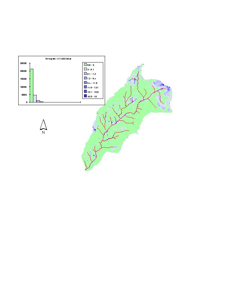
Figure 6. FS distribution (w=0, C=0.2)
The grid cells where FS£ 1under the best case are
depicted in black below.
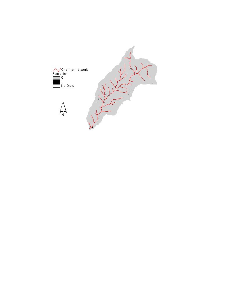
Figure 6. Grid cells where FS£ 1 (w=0, C=0.2)
The cells where FS£ 1 consist 0.225% of
the watershed. In a worst scenario 68% of the watershed was found to experience
FS£ 1, those are shown below in red.
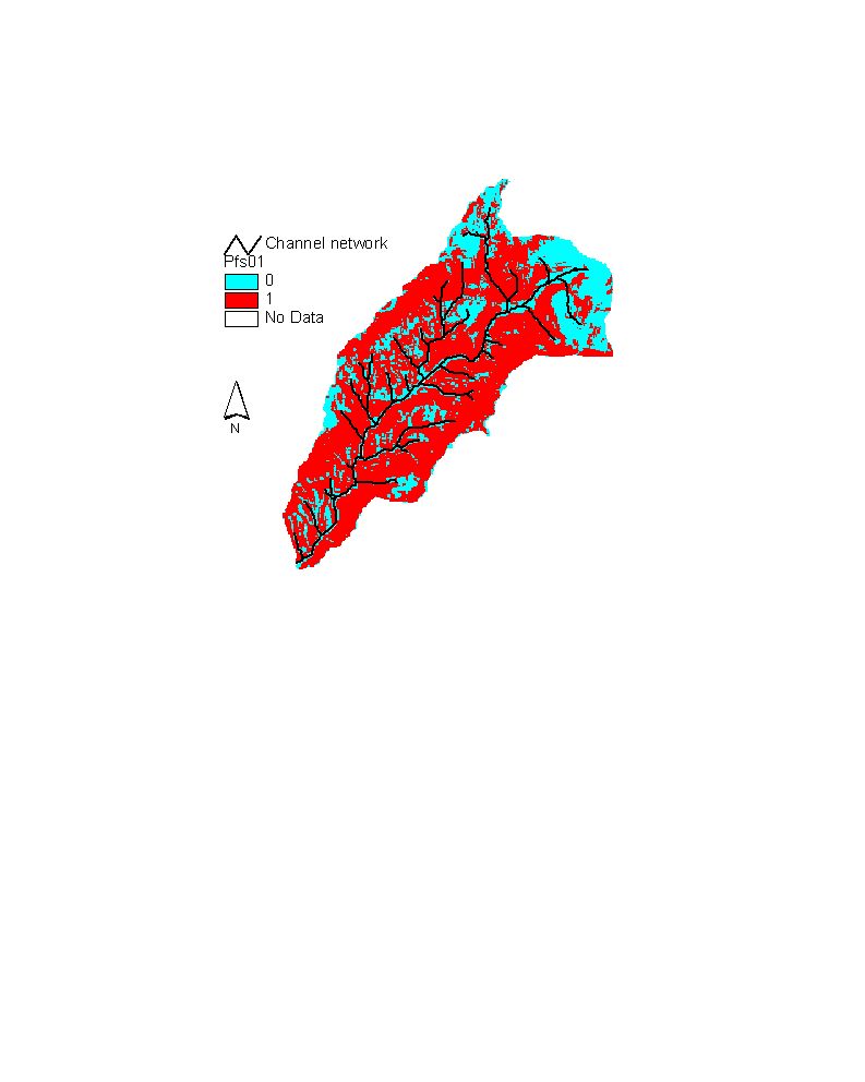
Figure 7. grid cells where FS£ 1 (w=1, C=0)
Also conditions for (w=0, C=0) and (w=1, C=0.2) are evaluated.
The watershed area (%) where FS£ 1 are found as 8.8%
and 17.4% respectively.
Threshold precipitation rates were calculated for both combined
cohesion conditions, (C=0 and C=0.2) by eqn.(13). After this calculation R
values which fall into the area of Fig7 were extracted. Because (13) can give an
R value which makes w£ 1, and if the cell do not yield
an FS£ 1 even w=1, then R value for those cells would
be the one with w=1.
The R values calculated for C=0 are given below.
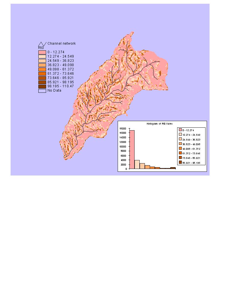
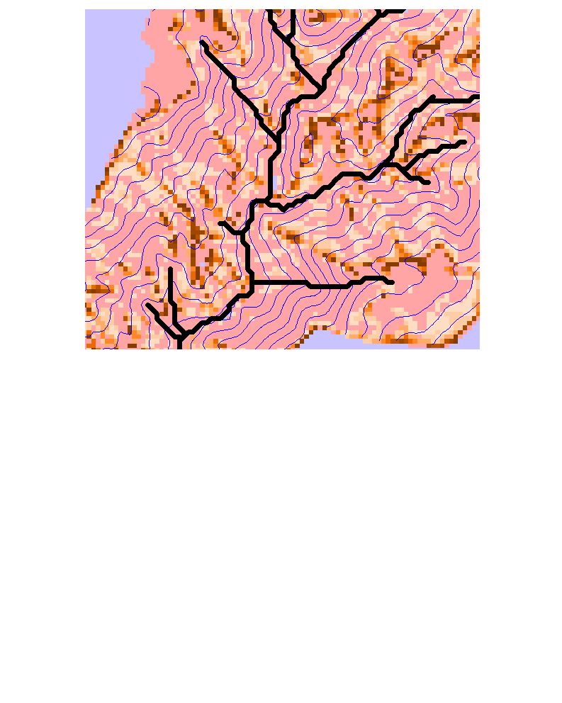
Figure 8. Threshold precipitation for slope stability (R)
distributed over the watershed when C=0, (a) the entire watershed (b) a portion
of the watershed DEM contours of 40 m interval are added
In the histogram above more than 16000 grid cells were assigned to the
precipitation rate range (0-12.274 mm/day). However for the reasons discussed
above approximately 32% of the watershed do not yield FS£ 1 even w=1. Those areas have totally 11572 grid cells, so
that this amount should be subtracted from the first column of the
histogram.
Threshold precipitation rates calculated for C=0.2 condition is given
below.
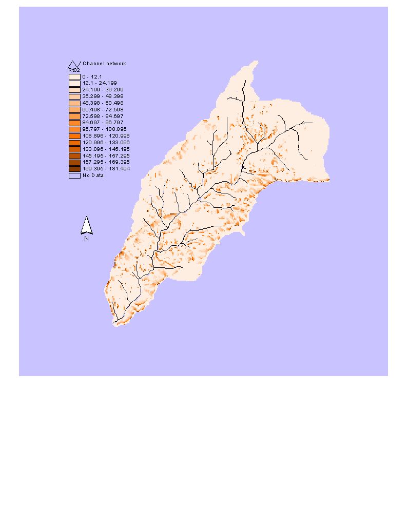
Figure 9. Threshold precipitation for slope stability (R) distributed over
the watershed (C=0.2)
In this condition 82.6% of the watershed, which correspond to 23515 grid
cells do not experience non-stabile conditions. Maximum precipitation for all
the grid cell which are susceptible to non-stabile conditions is 181 mm per day.
When C=0 in Fig(8) this value was approximately 110 mm per day. With this
example we can see how a small change in combined cohesion may affect the
threshold precipitation and total extend of non stable areas (see; Fig7, and the
paragraph below the figure).
Using the estimated values in the calculations above, functional
relationships between precipitation rate and probability of saturation and
non-stability were constructed. The probability concepts assumed are;
Probability of Saturation [Pr(Saturation)]= Areal percentage of the watershed
where saturation occurs under a given steady state precipitation rate.
Probability of non-stability [Pr(FS£ 1)]= Areal
percentage of the watershed where (FS£ 1) under a given
steady state precipitation rate
Figure given below shows the relationships discussed above.
Figure 10. Relationships between steady state precipitation rate and
probability of non-stability and saturation
Equations fit to those curves are;
Probability of saturation Pr(Sat.);
Pr(Sat.)= -2E-10R4 +2E-07R3 -9E-05R2 +
0.0149R+0.0545 (R2=1)
Probability of non-stability Pr(FS£ 1);
Pr(FS£ 1)=
1E-09R4-4E-07R3+3E-05R2+0.0011R-0.0003
(R2=0.9982) [C=0.2]
Pr(FS£ 1)=
8E-07R3-0.0002R2+0.0174R+0.0053 (R2=0.9998)
[C=0.0]
Application to Silver Creek
In Silver Creek average maximum snow melt water equivalent is 55cm. If we
assume that all this snow melts in one and a half month uniformly, then R would
be approximately 12 mm/day. Since a month time brings most of the watershed to
steady state conditions, than:
Pr(Sat.)= 0.185;
Pr(FS£ 1)= 0.16 [C=0]
Pr(FS£ 1)=0.025 [C=0.2]
CONCLUSION
These curves only give the general behavior of the watershed for saturation
and slope stability under steady state precipitation. They can be used to
calculate what portion of the watershed is saturated and/or non-stable for a
given steady state precipitation rate. Knowing the saturated portion is good to
roughly evaluate the erosion and sediment transport processes. The watershed
portion where (FS<1) may mobilize as landslides, but there is not a
certain criterion that I know, to identify the points to mobilize in the
watershed portion of FS<1. However the ones which have the minimum FS can be
assumed to mobilize. Threshold values for FS can also be considered and the ones
with lower FS would mobilize.
The uncertainty in the model parameters may be captured with the use of
curves. For a given precipitation rate, saturation level for both Pr(FS<=1)
curves is the same and the affects of the uncertainties in other parameters
(cohesion and internal friction angle) to the final probability can be observed.
The region between the two curves may give the probabilities of non-stability in
the watershed when c moves from 0 to 0.2.
FUTURE WORK
A future work would require to evaluate the uncertainty
associated with transmissivity and internal friction angle and develop curves
using those uncertain parameters and find out possible solution regions for
probability estimates.
References;
Barling, R.D., I.D., Moore and R.B., Grayson, 1994. A quasi-dynamic wetness
index for characterizing the spatial distribution of zones of surface saturation
and soil water content. J. of Water Resources Research, 30(4), 1029-1044.
Beven, K.J., and M.J. Kirkby, 1977. Considerations in the development and
validation of simple physical-based, variable contributing area model of basin
hydrology. Procc. of 3rd. International Symposium on Theoretical and
applied Hydrology, Colo. State Univ., Fort Collins, 1977.
Beven, K.J., and M.J. Kirkby, 1979. A physical-based variable contributing
area model of basin hydrology. Hydrol. Sci. Bull., 24, 43-69.
Beven , K., 1981. Kinematic subsurface stormflow, Water Resour. Res., 17(5),
1419-1424.
Dietrich, W.E., C.J., Wilson, D.R., Montgomery and J. M., Romy Bauer. 1992
erosion thresholds and landsurface morphology. J. Geology, (20): 675-679.
Dietrich, W.E., C.J., Wilson, and J. McKean, 1993, Analysis of erosion
thresholds, channel networks, and landscape morphology using terrain model. J.
of Geology, (101), 259-278.
Gray D.H and W.F. Megehan, 1985. Forest vegetation removal and slope
stability in the Idaho Batholith. Research paper INT-271, USDA Inter mountain
forest and range experiment station.
Megehan, W.F., S.B. Monsen and M.D. Wilson, 1991. Probability of Sediment
Yields From Surface Erosion on Granitic Roadfills in Idaho. J. of Env. Quality
(22)1, 53-60.
O'Loughlin, E. M., 1986. Prediction of surface saturation zones on natural
catchments by topographic analysis. Water Resour. Res., 22(5), 794-804.
Pack, R.T., D.G. Tarboton and C.N. Goodwin, 1998. Terrain stability Mapping
with SINMAP, technical description and users guide for version 1.00, Report
Number 4114-0, Terratech Consulting Ltd., Salmon Arm, B.C., Canada.
Wu, W., and R.C., Siddle, 1995. A distributed slope stability model for steep
forested basins. Water Resources Research, 31(8): 2097-2110.
Tarboton, D. G.,
(1997), "A New Method for the Determination of Flow Directions and Contributing
Areas in Grid Digital Elevation Models," Water Resources Research, 33(2):
309-319.