Exercise 3. Using Spatial Analysis to Calculate Area Average Precipitation
Prepared by Christina Bandaragoda and David Tarboton, Utah State University.
Table of Contents
· Goal
· Overview of what is to be done
· Computer and data requirements
1. Viewing grid data in ArcMap and examining data.
2. Adding tabular data and identifying associated grid data.
3. Calculation of Area Average Precipitation using Thiessen Polygons.
4. Using the field calculator to determine precise x and y coordinates.
5. Estimate basin average mean annual precipitation using Spatial Interpolation/Surface fitting.
Goal
The goal of the exercise is to serve as an introduction to Spatial Analysis with ArcGIS and learn how to analyze precipitation data and compute area average precipitation using data from a variety of data sources.
Overview of what is to be done
1. Display the watershed outline, state boundaries and Digital Elevation Model (DEM) in ArcMap. Create and display contours and hillshading from the DEM.
2. Convert tabular latitude and longitude data from reyprecip.txt to add to your map the display of raingage locations. Identify geographically, attributes of the raingage data. Report the rainfall and elevations associated with certain raingages.
3. Estimate basin average mean annual precipitation using Thiessen polygons by using the Spatial Analyst distance allocation function, then exporting the data into Excel for weighted averaging.
4. Use the field calculator to determine precise UTM projection x and y coordinates of points that were input in geographic coordinates.
5. Use the interpolation capability within Spatial Analyst to estimate mean annual precipitation surfaces using kriging or smoothing splines. Estimate basin average mean annual precipitation based on these surfaces.
6. Use the elevation at each precipitation gage to develop a relationship between elevation and mean annual precipitation. Use this relationship to estimate basin average mean annual precipitation (the Hypsometric method) accounting for topography.
Computer and Data Requirements
To carry out this exercise, you need to have access to a computer which runs ArcGIS, version 8.0 or later. You need the following data:
1. A shape file giving the outline of Reynolds Creek (rcout.shp).
2. A table of annual average rainfall data called reyprecip.txt.
3. A digital elevation model grid file called reydem.
4. A shape file giving the US State boundaries.
These data are in the file Ex3.zip (downloadable from the class web page). Unzip all the files into a single folder (directory), use the option checkbox Use Folder Names.
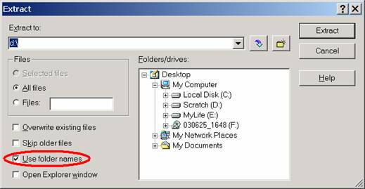
For illustrative purposes I will assume this directory is 'C:\rain\'. The files in the zipfile consist of the following files: rcout.shp, states.shp, reydem, reyprecip.txt. The files in bold are GIS files that physically comprise several files with different extensions. Do not concern yourself with this, just extract the whole zipfile, then you should have all the pieces you need and ArcGIS will see the multiple files as one.
1. Viewing data ArcMap and examining data
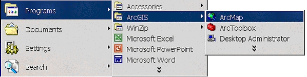
(1) Open ArcMap and select the "A new empty map" option.
(2) Use the ![]() (Add Data) button to Add Data. At the dialog that appears navigate to the folder, which
contains the data (c:\rain) and select the file rcout.shp. This is a shapefile giving the outline of Reynolds
Creek Experimental Watershed. This should be loaded first because it has
associated with it the UTM projection that the ArcMap Data frame will
inherit. (This projection information is
in the file rcout.prj.)
(Add Data) button to Add Data. At the dialog that appears navigate to the folder, which
contains the data (c:\rain) and select the file rcout.shp. This is a shapefile giving the outline of Reynolds
Creek Experimental Watershed. This should be loaded first because it has
associated with it the UTM projection that the ArcMap Data frame will
inherit. (This projection information is
in the file rcout.prj.)
(3) Add the states.shp data. Click OK to the
warning about a different geographic coordinate system. Click the ![]() (zoom to
full extent) button to see the
(zoom to
full extent) button to see the
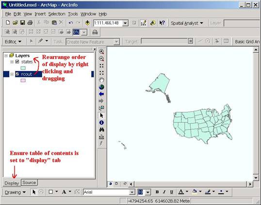
You should then see Reynolds Creek as a small dot in the south west corner
of ![]() (zoom in)
button then drag over this area to zoom in on the basin.
(zoom in)
button then drag over this area to zoom in on the basin.
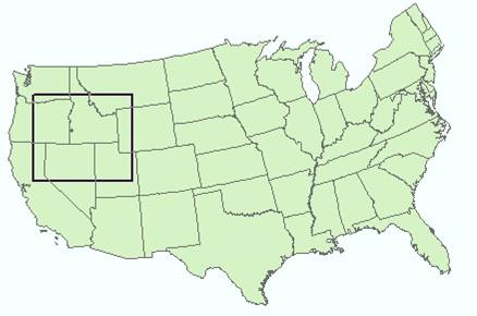
until you have a picture something like
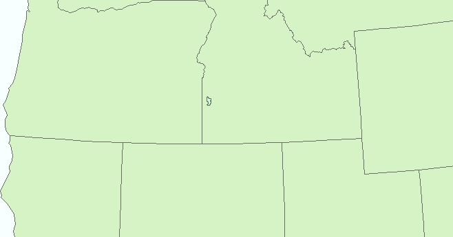
showing the location of the watershed in the SW corner of
This was just to show you where Reynolds Creek is and give an idea of scale.
(4) Save your work in ArcMap by choosing File/Save and selecting a file name (the file will be assigned extension mxd).
(5) Use the ![]() (Add
Data) button to add the digital elevation model raster "reydem". The added file is
listed in the Arc Map Table of contents.
(Add
Data) button to add the digital elevation model raster "reydem". The added file is
listed in the Arc Map Table of contents.
A raster or grid is a data structure that supports numerical values on a square grid. In this case the values represent topographic elevation. In ArcMap raster data is stored in an ESRI proprietary grid data structure comprising the principle folder (here named reydem), files inside it (which you do not need to concern yourself about) as well as *.aux files and files in the "info" folder. These should have been extracted in their entirety from the Ex3.zip data file. These files should not be manipulated except through Arc software (ArcMap or ArcCatalog). ArcCatalog is a utility similar to Windows explorer for managing GIS data. If you move one of the files in a raster folder, but not the other ones the raster may become corrupt and unusable.
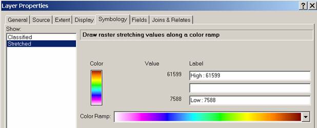
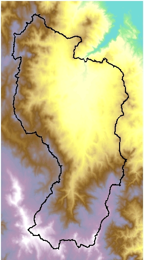
(6) Zoom right in over the watershed, turn the states layer off and adjust the rcout layer so that it is transparent so that the watershed outline is displayed relative to the DEM. You can recolor the raster by going to the theme's Properties/Symbology and choosing a new color ramp
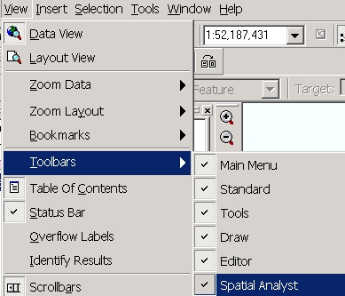
(7) Select Tools/Extensions.
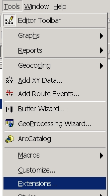
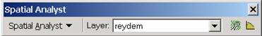
Make sure that "Spatial Analyst" is checked. Select View/Toolbars/Spatial Analyst to get the spatial analyst toolbar.
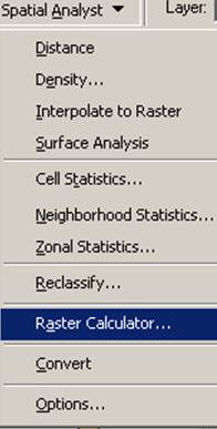
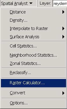
To explore the highest elevation areas in your DEM select Spatial Analyst/Raster Calculator.
The Raster Calculator, through the Map Algebra analytic capability it provides, is a major strength of Spatial Analyst. The Raster Calculator performs mathematical computations within and between raster datasets, raster layers, tables, and numbers and between valid combinations of them all. The set of operators is composed of arithmetical, relational, Boolean, bitwise, and logical operators that support both integer and floating-point values and combinatorial operators.
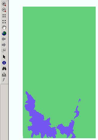
Double click on the layer reydem with the DEM for Reynolds Creek. Click on the > symbol and select a number less than the maximum elevation (2000 m). This arithmetic raster operation will select all cells with values above the defined threshold. In the example below a threshold of 2000 m was selected for the Z pixel value of reydem.
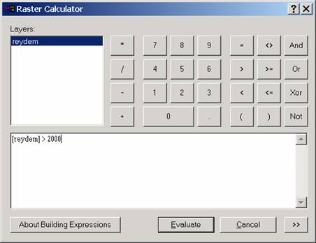
A new layer called calculation appears on your map. The majority of the map (green color) has a 0 value representing false (values below the threshold), and the blue region has a value of 1 representing true (elevations higher than 2000 m).
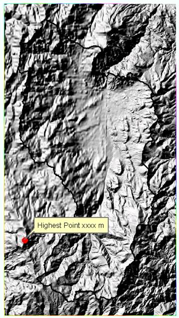
Zoom in to the region of highest elevations (blue region) and do some
sampling on the reydem grid using the identify ![]() tool to select a point close to the maximum
elevation. In a layout mark your point of maximum elevation and label it with
the elevation value for that pixel.
tool to select a point close to the maximum
elevation. In a layout mark your point of maximum elevation and label it with
the elevation value for that pixel.
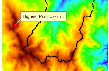
You can place the dot using the Draw toolbar. 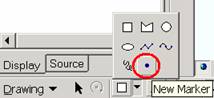
Contours
Contours are a useful way to visualize topography. This can be done using Spatial Analyst by doing the following:
Select Spatial Analyst > Surface Analysis > Contour
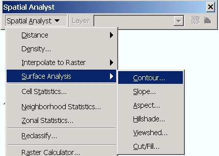
Set the contour interval to 100 m and name the output feature "cont100.shp"
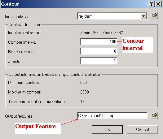
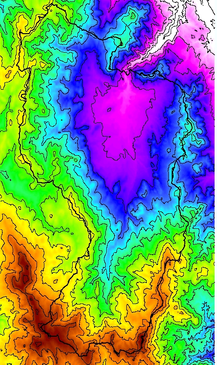
Click OK. You should see the cont100.shp file with 100 m contours on your map.
Another option to provide a nice visualization of topography is Hillshading. Select Spatial Analyst > Surface Analysis > Hillshade and set the factor Z to a higher value to get a dramatic effect and leave the other parameters at their defaults. Click OK. You should see and illuminated hillshaded view of the topography.
This shows some vertical and horizontal stripes in the data. This is indicative of poor interpolation in the joining of mapped blocks (This is an old dataset. This may have been corrected in the most recent National Elevation dataset).
1. To hand in. A layout
showing the outline and topography of Reynolds Creek and its location in the
2. Adding tabular data and identifying associated grid data.
The file reyprecip.txt contains annual average precipitation data for 25
stations in Reynolds Creek, with their coordinates. This data is described in (Hanson, C. L.,
(2001), "Long-Term Precipitation Database, Reynolds Creek Experimental
Watershed,
(1) Use the ![]() (Add Data) button to add the data table "reyprecip.txt". This file
should then appear in the table of contents (source tab) of the active data
frame, but not on the map, because the system does not (yet) know how to
interpret the data geographically.
(Add Data) button to add the data table "reyprecip.txt". This file
should then appear in the table of contents (source tab) of the active data
frame, but not on the map, because the system does not (yet) know how to
interpret the data geographically.
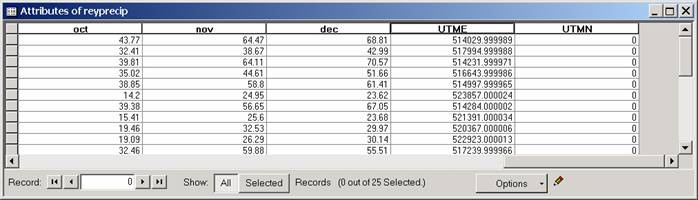
(2) Right click on this table of contents entry and select Open
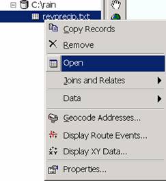
This displays in tabular form the data read from file reyprecip.txt.
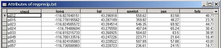
Note that there are fields named long and lat that give the locations of the precipitation stations in geographic coordinates. Close the table.
Right click on Layers/Properties
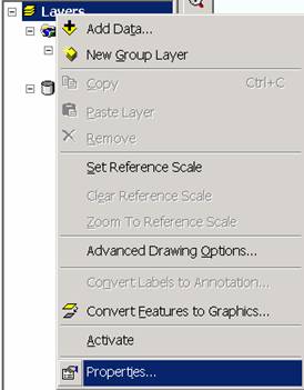
then on the Coordinate System tab
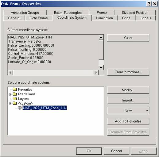
This shows that the data frame (named Layers) is using NAD 1927 UTM zone 11 coordinates. To display the precipitation gages correctly they need to be plotted using this coordinate system. Click OK or Cancel to close the Data Frame Properties dialog.
(3) Right click on the table of contents entry for 'reyprecip.txt' and select display XY data.
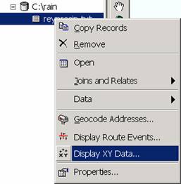
At the display XY data dialog adjust the X field to long and Y field to lat. Click on Edit to set the Coordinate System. Select a predefined coordinate system and browse to Geographic Coordinate Systems/North America/North American Datum 1927.
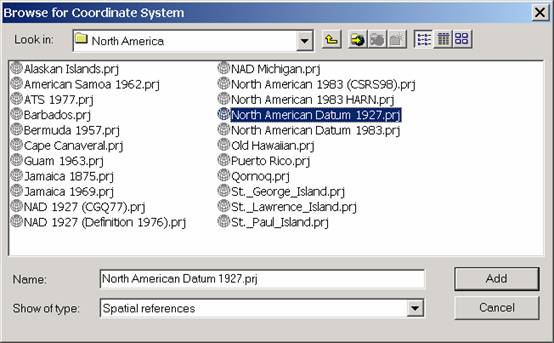
Click Add, then at the Spatial
Reference Properties dialog, OK
The Display XY Data dialog should now display the coordinate system selected
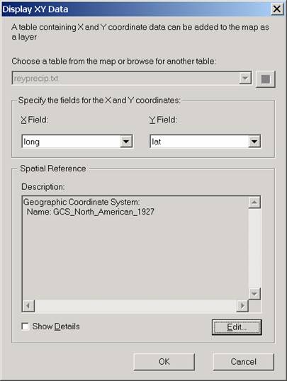
Click OK. The raingage locations should now be displayed on the map. Change the symbology of these to something that depicts raingages.
(4) In addition to being useful for the display of geographic data,
GIS is useful for the querying of numerical and text attribute data associated
with the geographic data items. The identify features tool ![]() on the "Tools" toolbar is used to display attribute data of features
in the Map by clicking on them. Click on
the Identify Features tool
on the "Tools" toolbar is used to display attribute data of features
in the Map by clicking on them. Click on
the Identify Features tool ![]() , then Click on the
location on the map you are interested in, and in the Identify Results
window select the object you are interested in.
, then Click on the
location on the map you are interested in, and in the Identify Results
window select the object you are interested in.
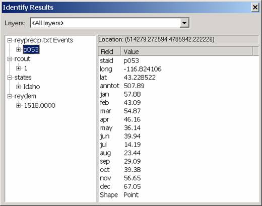
For example the above display indicates that the station identifier 'staid'
of the gage I clicked on was P053, the annual precipitation 'anntot' at this
location was 507 mm (The units need to be ascertained independently of the
database). The elevation from the DEM is
1518 m, and this is in the state
2. To hand in. Report the Station Identifier (staid), elevation and mean annual precipitation at the northernmost, and westernmost raingages in this dataset.
3. Calculation of Area Average Precipitation using Thiessen Polygons
Now to do something useful. We will calculate the area average mean annual precipitation over the watershed using Thiessen polygons.
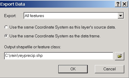
(1) Preparation of rain gage shapefile. Convert the reyprecip.txt events display to a shapefile. Right click on "reyprecip.txt events" and select Data/Export Data.
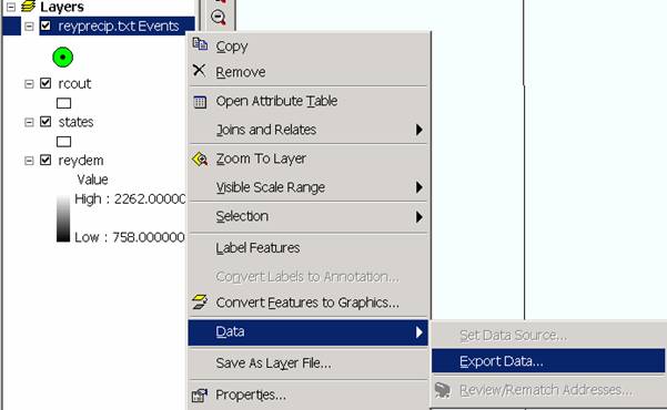
At the export data dialog, click use the same coordinate system as the data frame (to convert from latitude and longitude to UTM coordinates) and specify the output name "reyprecip.shp"
Click "Yes" to add the exported layer to the map. Right click and open the attribute table of the shapefile just added
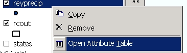
Note that the first attribute is FID (Feature Identifier). This attribute was not present in reyprecip.txt events. This attribute is necessary for the next step where we associate a Thiessen polygon with each raingage.
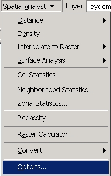
(2) Preparation of Spatial Analyst. The calculations are done using Spatial Analyst. First set the options of Spatial Analyst to cover the domain of interest. Click on Spatial Analyst/Options.
On the general tab set the working directory to your working directory "C:\rain", analysis mask to "rcout" the outline of the watershed, and coordinate system to the same as the active data frame (This should be UTM inherited from rcout.shp).
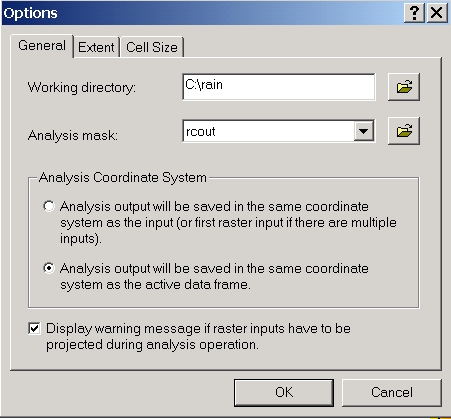
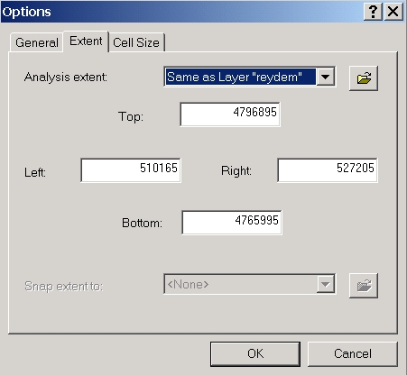
Don't click OK just yet. On the Extent tab set the Analysis extent to same as layer "reydem".
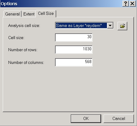
On the Cell Size tab set the Cell size to same as layer "reydem"
Now you can click OK.
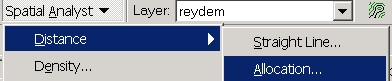
(3) Thiessen Polygons. Thiessen polygons associate each point in a watershed with the nearest raingage. In GIS terminology this is an "allocation" function based on distance. Click on Spatial Analyst/Distance/Allocation
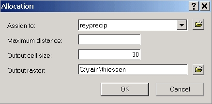
At the Allocation dialog make sure that the Assign to field is reyprecip (the raingage shapefile) and give the output raster a name "thiessen".
Click OK. The result should be a grid "thiessen" that looks like
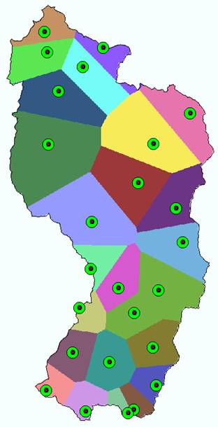
This has formed a grid that has the value of the FID of the nearest rain gage at each location within the watershed (analysis mask). This effectively associates with each 30 m grid cell within the watershed the nearest raingage. Look at (Right click then Open) the attribute table of the new grid "thiessen". It contains attributes, Object ID, Value and Count. The Object ID corresponds to the FID in the reyprecip attribute table. The count (times grid cell size) gives the area within the watershed assoicated with each raingage. These tables need to be joined to do the area weighted average precipitation calculation. Right click on thiessen and select Joins and Relates/Join.
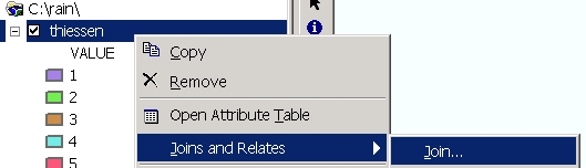
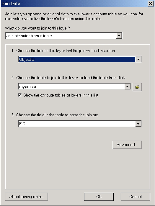
Choose the field in this layer that the join will be based on: "ObjectID" (in thiessen attribute table). Choose the table to join to this layer: "reyprecip" and choose the field in the table to base the join on: "FID".
Click OK. Now open the attribute table of thiessen. Note that the attributed of reyprecip are now included in this table. Export this table so that the area weighting calculation can be done in Excel. Click on Options/Export
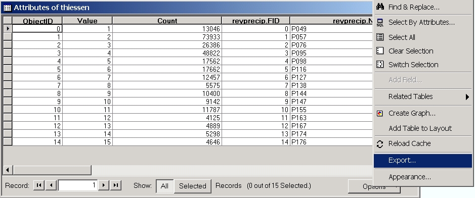
Name the output file "thiessen.dbf". There is no need to add this to the map. Now open the "thiessen.dbf" file from Excel. Use the Count (Column C, representing the number of grid cells associated with each polygon) and anntot (Column H, representing the annual precipitation in mm at the gage) to calculate the area average precipitation.
3. To hand in. A layout showing the Thiessen polygons.
Report the station identifier of the precipitation gage that is associated with
the largest Thiessen polygon. Report the
4. Using the field calculator to determine precise x and y coordinates.
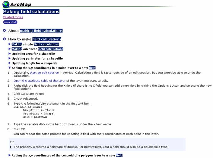
The work above included a coordinate transformation from geographic coordinates to UTM coordinates for precipitation gage locations. It is frequently handy to have these coordinates in a table, for example to provide as coordinates to a third party statistical program for interpolation. To see how to do this click on ArcMap Help and search for 'making field calculations'. Expand the text about adding the x,y coordinates in a point layer to a new field to see the following display
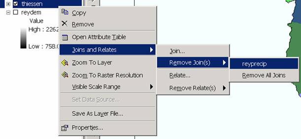
We will next step through this procedure to add two new fields UTME and UTMN to the attribute table reyprecip shape file. This can not be done while the attribute table is in use in a join so first right click on the thiessen layer and select to remove the reyprecip join.
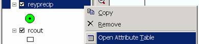
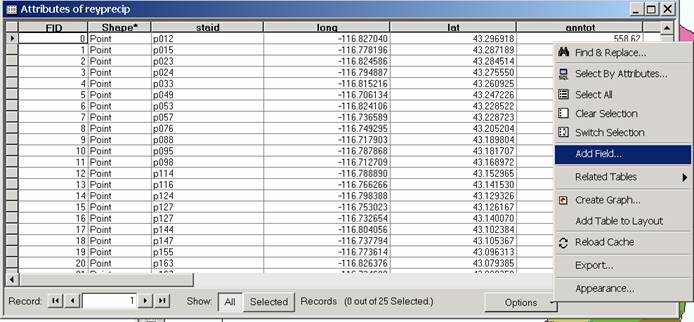
Then open the reyprecip attribute table
Click on Options/Add field.
Sometimes it is necessary to close and reopen ArcGIS if it thinks the table is still in use.
Name the field being added UTME, with type double.
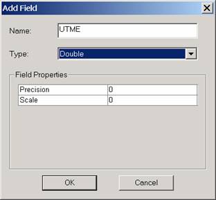
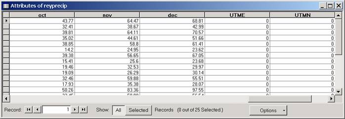
Click OK. Notice that a new field has been appended on the right of the attribute table. Add another field UTMN, also of type double. The right of the attribute table should now look like
Click Editor/Start Editing (This start editing step is strictly not necessary but is advisable if you want to be able to undo your work if you make an error).
![]()
Indicate the folder containing the reyprecip shapefile.
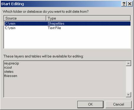
Click OK.
The appearance of a little pencil next to the options button reminds you the shapefile is being edited.
![]()
Right click on the UTME header and click Calculate Values
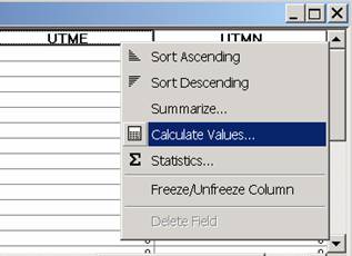
This brings up the Field Calculator tool.
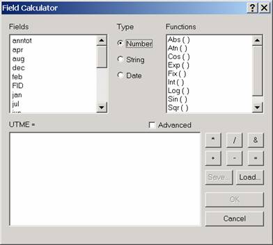
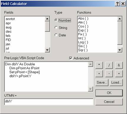
This is a general purpose tool that allows one to do algebraic like operations on fields in a table. This could have been used with the thiessen table above to calculate the Thiessen Polygon area average rainfall, but it is usually easier to use Excel. Here we will use the advanced capability of this tool to run VBA script. Click on Advanced. Copy the code from the Making Field Calculations help into the fields so that you end up with

Click OK. The X coordinates (UTM eastings) should appear in the table in the attribute field UTME.
Now do the same for UTMN, except modify the code to get the point Y values from the shape.
Your table should now have both X and Y UTM coordinate values for each of the precipitation gages.
Select Editor/Stop editing
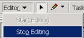
Click Yes to save edits.
Export the edited attribute table of reyprecip (or just use Excel to open reyprecip.dbf) and prepare a table giving the Station Identifier (staid), Latitude, Longitude, and UTM coordinates (X and Y) for these 25 precipitation stations. This should look something like
|
staid |
long |
lat |
UTME |
UTMN |
|
p012 |
-116.827040 |
43.296918 |
514030.00 |
4793587.00 |
|
p015 |
-116.778196 |
43.287189 |
517995.00 |
4792516.00 |
|
p023 |
-116.824586 |
43.284514 |
514232.00 |
4792210.00 |
|
... |
... |
... |
... |
... |
Use the UTM coordinates to calculate the distance between stations p012 and
p17607. Use the measure tool ![]() to check your result. Which do you think is more accurate?
to check your result. Which do you think is more accurate?
4.
To hand in. A table showing the
Station ID, Longitude, Latitude, UTME and UTMN of each precipitation gage. Report the distance between stations p012 and
p17607.
5. Estimate basin average mean annual precipitation using Spatial Interpolation/Surface fitting.
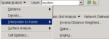
Thiessen polygons were effectively a way of defining a field based on discrete data, by associating with each point the precipitation at the nearest gage. This is probably the simplest and least sophisticated form of spatial interpolation. ArcGIS provides other spatial interpolation capabilities under the Spatial Analyst/Interpolate to raster functions.
We will not, in this exercise, concern ourselves too much with the theory behind each of these methods. You should however be aware that there is a lot of statistical theory on the subject of interpolation, which is an active area of research. This theory should be considered before practical use of these methods.
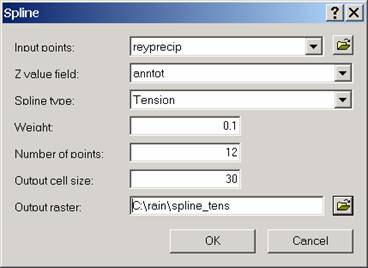
For this exercise I suggest you just try a few of the methods, examining the surface that results to see if you like them. Some options do not work due to insufficient data to estimate the necessary variogram (a statistical function quantifying the spatial dependence used as a basis for kriging interpolation) and some options result in negative precipitation. Use the input points from "reyprecip" and Z value field as "anntot".
Following is how I set up a tension spline interpolation.
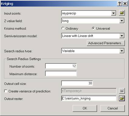
Following is how I set up a Kriging interpolation. I was unable to get ordinary Kriging to work with this data. There are insufficient data points to estimate a variogram (it says).
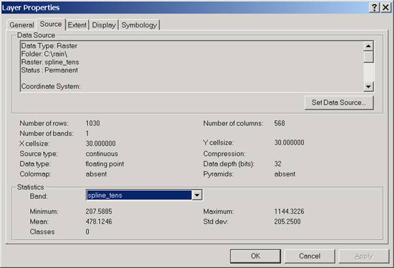
To obtain the mean of an interpolated surface right click on it and select Properties. Select the Source tab to examine the mean (and other statistics). The mean is the area average precipitation from the spatially interpolated surface.
Some interpolation functions, notably Kriging, do not limit the result to the analysis mask. In these cases to isolate the area being averaged to the watershed a raster calculation needs to be used. Select Spatial Analyst/Raster Calculator.
At the dialog complex algebraic calculations on layers can be performed. Here we just need to double click on the layer of interest, "kriging" so that it appears in the building expressions box below then click evaluate.
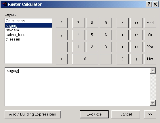
The result should be a layer that conforms to the analysis mask. This works because the analysis mask for Spatial Analyst was set earlier. The properties/Source tab on the layer that results displays statistics.
5. To hand in. A layout showing the interpolated mean annual precipitation surface over Reynolds Creek. Report what method you used. Report the basin average mean annual precipitation from the "anntot" attribute, as well as minimum, maximum and standard deviation for this within the basin area (i.e. the analysis mask must have been set using rcout.shp).
6. Estimation of area average mean annual precipitation by the Hypsometric method using a precipitation versus elevation relationship.
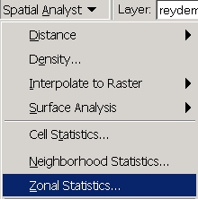
The elevation values associated with each precipitation gage may be determined automatically using the Spatial Analyst/Zonal Statistics function
Set the Zone dataset to "reyprecip" (this is the dataset defining the locations for which statistics are to be evaluated), the zone field as "staid" (a unique field in reyprecip to join the table produced to reyprecip). Uncheck the Chart statistic and Check the Join output table to zone layer. Choose an output table name that you like (or stick with the default).
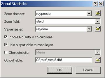
Click OK. The table that appears shows the minimum, maximum, mean, range ... of the elevation field associated with each object in "reyprecip". Because reyprecip.shp is a point shape file the minimum, mean, etc are all the same. Had reyprecip.shp been a polygon or line shape file these would have been statistics over the space covered by the polygons or lines. Close the table that appears. Open the attribute table associated with "reyprecip". Because the "Join output table ..." was selected the zone statistics have been added to this table. Use Options/Export on this table to save it as a DBF table named rainelev.dbf. There is no need to add this to ArcGIS.
Open the rainelev.dbf table using Excel. Develop a relationship between total precipitation (i.e. anntot in column d) and one of the fields representing elevation (e.g. Mean in column AA)
Now use Spatial Analyst/Raster Calculator to compute a raster of precipitation based upon elevation data and this relationship, e.g. ([Reydem] * 0.772 - 696)
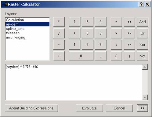
Use Properties/Source to examine the mean of the result.
6. To hand in. A layout showing the mean annual precipitation surface over Reynolds Creek estimated from elevation. Report the basin average precipitation (mean in mm from the "anntot" attribute), as well as minimum, maximum and standard deviation for this within the basin area (i.e. the analysis mask must have been set using rcout.shp). Report your precipitation vs elevation relationship.
Summary of Material to be Turned In
1. A layout showing the outline and topography of Reynolds Creek
and its location in the
2. Report the Station Identifier (staid), elevation and mean annual precipitation at the northernmost, and westernmost raingages in this dataset.
3. A layout showing the Thiessen polygons. Report the
station identifier of the precipitation gage that is associated with the
largest Thiessen polygon. Report the
4. A table showing the Station ID, Longitude, Latitude, UTME and
UTMN of each precipitation gage. Report
the distance between stations p012 and p17607.
5. A layout showing the
interpolated mean annual precipitation surface over Reynolds Creek.
Report what method you used. Report the basin average mean annual
precipitation from the "anntot" attribute, as well as minimum,
maximum and standard deviation for this within the basin area (i.e. the
analysis mask must have been set using rcout.shp).
6. A layout showing the mean annual precipitation surface over Reynolds Creek estimated from elevation. Report the basin average precipitation (mean in mm from the "anntot" attribute), as well as minimum, maximum and standard deviation for this within the basin area (i.e. the analysis mask must have been set using rcout.shp). Report your precipitation vs elevation relationship.