Application of ArcGIS 8

Utah is in the western mountainous region; topography varies greatly, elevation changes from about 600 to over 4000 m, and many kinds of vegetation exist here. On the other hand, weather stations are limited in number and only offer local data, i.e., point data, of meteorological conditions. In plain regions, these point data from weather stations can be directly used to represent conditions in some range of area. But in the region such as Utah with so much varied topography, it is difficult to use these point data to represent area situation. ArcGIS 8.1 offers tools for spatial analysis, which can be used to interpolate point data to grid data. In this term project, spline methods of interpolation offered by ArcGIS 8.1 were compared and applied to create climate conditions scenarios in the range of all Utah, then climate conditions in different vegetation zones were analyzed and compared.

2. DATA RESOURCES

Data of vegetation distribution in Utah, climate data of annual average temperature and annual precipitation at weather stations, and DEM of Utah are used in this project. Data of vegetation distribution in Utah is from the website of Automated Geographic Reference Center, Division of Information Technology Services, Utah (http://agrc.utah.gov/sgid/statewide/index.htm). It is in Arc/Info interchange file format. This dataset, published on Jan 1, 1987, represents the statewide distribution of dominant vegetation species in Utah with a coordinate system of Clarke_1866_UTM_Zone_12N, for regional analysis and display at 1:500,000.

Climate data of Utah are from website (http://wrcc.sage.dri.edu/summary/climsmut.html) of Western Regional Climate Center. It offers climate summaries of 223 weather stations in Utah, which include station position description, period of records, annual and monthly extreme and average temperature, annual and monthly precipitation, and other data. In this project, data of station position, annual average temperature, and annual precipitation were mainly used.

DEM of Utah is from Mr. Shujun Li, a student of Utah State University. He got DEM of different districts in Utah from USGS and merged them into one for whole Utah with a resolution of 90 m.

3. METHODS FOR DATA PROCESSING

3.1. Re-classification of Vegetation Distribution

The file of vegetation distribution downloaded is in Arc/Info interchange file format. Its shapefile can be got with Import to Coverage/Import from Interchange File and Export from Coverage/Coverage to Shapefile under the Conversion Tools in ArcToolbox.

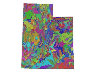
Figure 1 shows vegetation distribution in Utah from the original shapefile. It contains 57 dominant species of vegetation and non-vegetation, and totally 1270 polygons. It is TOO detailed for this project. These dominant species are regularly encoded on the basis of vegetation types (see Table 1), although the attribute table of the original shapefile does not involve the field of the code for the types.

Figure 1. Vegetation distribution in Utah from original shapefile.

Table 1. Code ranges of dominant species

Type	Dominant Species	Code Range
	Uncoded	0
Conifer - Aspen	Aspen, Douglas Fir, Utah Juniper, …	101 - 199
Mountain Brush	Maple, Mt. Mahogany, Oak, …	201 - 299
Herbs - Shrubs	Greasewood, Sagebrush, Shadscale, …	301 - 399
Grasses - Sedges	Cheatgrass, Saltgrass, Wheatgrass, …	401 - 499
River Bottom	Fremont Cottonwood, Narrowleaf Cottonwood, …	501 - 599
Cultural Forms	Cities	601
Cultural Forms	Cultivated Land	602
Physical Forms	Mud, Sand, Water, …	701 - 799

With the help of dissolving function in Tools/GeoProcessing Wizard…, vegetation types were re-classified. This needed to use dissolving function twice. The first was to merge the different polygons of the same dominant species. The procedures were:

(1) Select Tools/GeoProcessing Wizard … in ArcMap. GeoProcessing Wizard window appears.

(2) In the window, select Dissove features based on an attribute, and click Next.

(3) In the following window, Select the input layer to dissolve as vgdis.shp which is the original shape file of vegetation distribution, Select an attribute on which to dissolve as CODE, and Specify the output shapefile of feature class as vgdisDissove_1.shp, then click next.

(4) In the following window, choose AREA and check the checkbox before sum to calculate the area of each dominant species, which will be included in the output shapefile of feature class. Then click Finish.

The attribute table of the output shapefile is shown as Figure 2. It can be seen that vegetation had been dissolved to 57 dominant species plus one uncoded with CODE as 0. Use Editor tool in ArcMap to change the numbers in field CODE according to Table 2. Here I put cities and physical forms as well as uncoded areas into one type, non-vegetation.

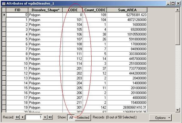
Figure 2. The attribute table of the output shapefile after the first dissolving of vegetation distribution

Table 2. Codes of vegetation types

Type	Code of Type	Code Range of dominant Species
Uncoded	0	0
Conifer - Aspen	100	101 - 199
Mountain Brush	200	201 - 299
Herbs - Shrubs	300	301 - 399
Grasses - Sedges	400	401 - 499
River Bottom	500	501 - 599
Cities	0	601
Cultivated Land	602	602
Physical Forms	0	701 - 799

Then do dissolving again to the output shapefile vegdisDissolve_1.shp, using the same procedures as shown above. Vegetation distribution based on types would be output.

3.2. Climate Conditions

3.2.1. Choose Weather Stations

The website (http://wrcc.sage.dri.edu/summary/climsmut.html) offers climate data of 223 weather stations in Utah. But the periods of these climate data differ from one another very much. Table 3 shows that the beginning year for climate data differs up to 127 years, ending year does up to 46 years, and the shortest period is just 8 years while the longest is 139 years. So these data are not comparable.

Table 3. Difference in periods for climate data among weather stations in Utah

From Year		To Year		Duration (years)
Earliest	Latest	Earliest	Latest	Shortest	Longest
1864	1991	1954	2000	8	139

Stations with climate data from 1928~59 to 2000 were chosen, considering periods for climate data and number and distribution of stations. There are 75 stations chosen and their distribution is shown in Figure 3.

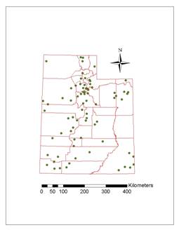
Figure 3. Distribution of chosen weather stations

3.2.2. Create Point Shapefile of Chosen Weather Stations

A shapefile of weather stations could be created in this way. First, build up with Excel a database file of station name, position (latitude, longitude, and elevation), annual average temperature, and annual precipitation data. Then, create the shapefile using Display XY Data… and Data/Export… functions in ArcMap.

3.2.3. Interpolate Point Data of Climate Conditions to Grid Data

Now, the point data of climate conditions could be interpolated into grid data, using Spatial Analyst/Interpolate to Raster /Spline… function. Spline estimates values using a mathematical function that minimizes overall surface curvature, resulting in a smooth surface that passes exactly through the input points. This method is best for gently varying surfaces such as elevation, water table heights, or pollution concentrations. There are two Spline methods: Regularized and Tension. The Regularized Spline type ensures that you create a smooth surface and slope. The Tension Spline type tunes the stiffness of the surface according to the character of the modeled phenomenon. The procedures to create a surface using Spline interpolation are:

(1) Click the Spatial Analyst dropdown arrow, point to Interpolate to Raster, and click Spline.

(2) Click the Input points dropdown arrow and click the point dataset you wish to use.

(3) Click the Z value field dropdown arrow and click the field you wish to use.

(4) Click the Spline type dropdown arrow and click the Spline method you wish to use.

(5) Optionally, change the default Weight. For the Regularized method, the higher the weight, the smoother the surface; typical values are 0, .001, .01, .1, and .5. For the Tension method, the higher the weight, the coarser the surface; typical values are 0, 1, 5, and 10.

(6) Optionally, change the default number of points to use in the calculation of each interpolated point. The more input points you specify, the more each cell is influenced by distant points and the smoother the surface is.

(7) Optionally, change the default output cell size.

(8) Specify a name for the output or leave the default to create a temporary dataset in your working directory.

(9) Click OK.

Both Regularized and Tension Spline methods were tried to interpolate annual average temperature and annual precipitation with default Weight (0.1), default Number of points (12), and output cell size was set as 500. They were also tried with some other Weight values.

3.2.4. Consider Elevation when Interpolating

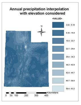
When point data of annual average temperature and annual precipitation were interpolated to grid data, elevation was considered. Figure 4 shows the relationship between annual average temperature and elevation of the 75 chosen weather stations. It can be seen that apart from one station, annual average temperature decreases as elevation increases; lapse rate is about 6 °C/km. The annual precipitation has a positive correlation with elevation (see Figure 5). Averagely, annual precipitation increases about 11.9 inches as elevation increases 1000 m. 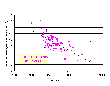While the elevation in Utah changes very much from about 600 m to more than 4000 m (see Figure 6), both temperature and precipitation difference due to elevation could be great.

Figure 4. Relationship between annual average temperature and

elevation of the 75 chosen weather stations

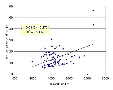
Figure 5. Relationship between annual precipitation and

elevation of the 75 chosen weather stations

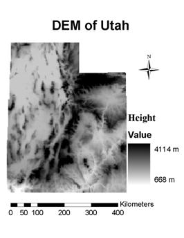
Figure 6. DEM of Utah

The method used for interpolation annual average temperature with elevation combined is:

(1) Convert station temperature into some level of the same elevation (here I used mean sea level), when building up .dbf file.

T_MSL,
point (ºC) = T_point (ºC) + elev(m) * 6 (ºC) / 1000(m)

(2) Interpolate T_{MSL, point} into grid data with Spline interpolation.

(3) Covert T_{MSL, grid} into surface data with Raster Calculator… function in Spatial Analyst, based on DEM data.

T_grid (ºC) = T_{MSL, grid} (ºC) – elev(m) * 6 (ºC) / 1000(m)

Similarly, the method for annual precipitation interpolation is:

(1) Convert station precipitation into some level of the same elevation (here I also simply used mean sea level), when building up .dbf file.

P_MSL,
point (in.) = P_point (in.) - elev(m) * 11.9 (in.) / 1000(m)

(2) Interpolate P_MSL into grid data with Spline interpolation.

(3) Covert P_MSL grid data into surface data with Raster Calculator… function in Spatial Analyst, based on DEM data.

P_grid (in.) = P_{MSL, grid} (in.) + elev(m) * 11.9 (in.) / 1000(m)

3.2.5. Zonal Statistics of Elevation and Climate Conditions in Different Vegetation Zones

Elevation and climate conditions of different vegetation types were statistically analyzed, with Zonal Statistics… function in Spatial Analyst. The Zonal Statistics function allows you to compute statistics for each zone of a zone dataset based on the information in a value raster. In this project, the zone dataset is the vegetation distribution, and the value raster is the grid dataset of elevation, annual average temperature, or annual precipitation. The procedures to use Zonal Statistics are:

(1) Click the Spatial Analyst dropdown arrow and click Zonal Statistics.

(2) Click the Zone dataset dropdown arrow and click the layer you want to use.

(3) Click the Zone field dropdown arrow and click the field of the Zone layer you wish to use.

(4) Click the Value raster dropdown arrow and click the raster you wish to use.

(5) Uncheck Ignore NoData in calculations to use the Nodata values of the value raster in the calculation.

(6) Check the checkbox to join the output table to the zone layer. Note: this option this only available for layers, not datasets you browse to.

(7) Click the Chart statistic dropdown arrow and click the type of statistic you wish to chart.

(8) Specify a name for the output table or leave the default to create a table in your working directory.

(9) Click OK.

4. RESULTS

4.1. Vegetation Distribution

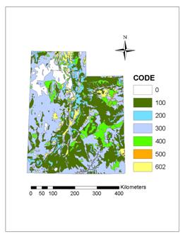
Distribution of different type vegetation is shown in Figure 7 and their area values are listed in Table 4. It can be seen that Herbs – Shrubs and Conifer – Aspen are two main types of vegetation in Utah; they totally cover about 72% of Utah. The other types cover about 5-9% each, except for River Bottom which only covers 0.4%. Comparing Figure 7 of vegetation distribution with Figure 5 of DEM, it is clear that vegetation of Conifer – Aspen is mainly located on mountains with higher elevation, while vegetation of Herbs – Shrubs is located at areas with lower elevation.

Figure 7. Distribution of different type vegetation

Table 4. Area comparison among different type vegetation

Type	Vegetation	Area (km^2)	Percent (%)
100	Conifer - Aspen	76472	34.7
200	Mountain Brush	12418	5.6
300	Herbs - Shrubs	82996	37.7
400	Grasses - Sedges	19865	9.0
500	River Bottom	827	0.4
602	Cultivated Land	11349	5.2
0	Non-vegetation (cities, water, sand, mud, …)	16371	7.4

4.2. Comparison between Interpolation with and without Elevation Considered

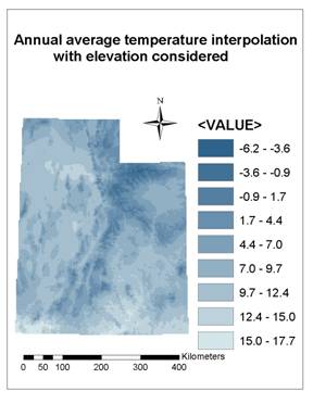
Figure 8(a) and (b) show grid data of annual average temperature interpolated from point data of the 75 chosen weather stations, with and without elevation considered, respectively. It can be seen that, with elevation considered, results of grid temperature is more reasonable; they can reflect the rule of temperature changing with elevation. Grid data in Figure 8(b) is blurred comparing to Figure 8(a), and the lowest temperature in Figure 8(b) is much higher than in Figure 8(a), both of which indicate that the interpolating method without elevation considered couldn’t got correct grid data, especially when the elevation of the grid being estimated is out of the range of elevations of surrounding sample points.

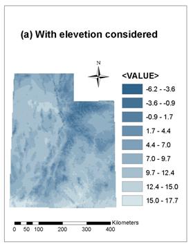
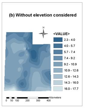
Figure 8. Annual average temperature interpolated with Tension Spline method and Weight taken as 0.1

(a) with elevation considered (b) without elevation considered.

4.3. Comparison between Regularized and Tension Spline Methods with Different Weight

There are two Spline methods: Regularized and Tension. For the Regularized method, the higher the weight, the smoother the surface; typical values are 0, .001, .01, .1, and .5. For the Tension method, the higher the weight, the coarser the surface; typical values are 0, 1, 5, and 10. Figure 9 gives the results of interpolating annual average temperature with both Regularized and Tension Spline methods. Different Weight values were taken for comparison: default (0.1) and 5 for Tension method, and default (0.1) and 0 for Regularized method. Elevation was considered in all the four cases. We can see that there is little difference between results with the Weight of 0.1 and 5 for Tension method (see Figure 9a and 9b), but huge difference exists between the results with the Weight of 0.1 and 0 for Regularized method (see Figure 9c and 9d).The result with the Weight of 0 for Regularized method (Figure 9d) is similar to those of Tension method, while the result with the Weight of 0.1 for Regularized method (Figure 9c) is unacceptable. This indicates that Tension Spline method may be more suitable for interpolating point data of climate conditions into grid data.

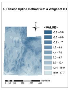
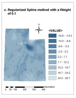
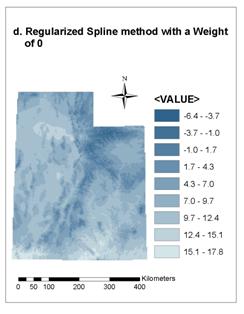
Figure 9. Results of the Regularized and Tension Spline method with different

Weight values for interpolating annual average temperature

4.4. Elevation and Climate Conditions in Different Vegetation Zones

Table 5 shows the statistical results of elevation and climate conditions in different vegetation zones. Here, annual average temperature and annual precipitation interpolated with Tension Spline method with default weight value of 0.1 (see Figure 10), were used. It seems regularity is not obvious from the extreme values (MIN and MAX) of elevation and climate conditions in Table 5. But from average values (also see Figure 11), Conifer-aspen and mountain brush are averagely located at higher elevation with lower annual average temperature and more annual precipitation, while vegetation of herbs-shrubs, grasses-sedges, and river bottom is contrary. Cultivated lands are specially located at lower elevation with higher temperature and more precipitation.

So vegetation in Utah could be roughly divided into three classes: the first class contains conifer-aspen and mountain brush, the second includes herbs-shrubs, grasses-sedges, and river bottom, and the third is cultivated land.

Table 5. Statistical results of elevation and climate conditions in different vegetation zones

	Elevation (m)				annual average temperature (˚C)				annual precipitation (in.)
Vegetation Type	MIN	MAX	MEAN	STD	MIN	MAX	MEAN	STD	MIN	MAX	MEAN	STD
Non-vegetation	779	3608	1331	174	-3.4	17.5	11.2	1.7	2.4	39.1	15.2	7.4
Conifer_Aspen	914	3914	2190	439	-5.7	16.6	6.3	3.5	3.1	63.2	16.4	5.9
Mountain Brush	1358	3381	2208	281	-2.7	13.1	5.4	2.3	7.1	61.4	21.0	5.7
Herbs_Shrubs	692	3048	1593	279	-1.9	17.7	9.9	2.6	2.4	38.3	10.7	4.4
Grasses_Sedges	1191	4031	1744	521	-6.2	14.5	8.5	3.4	3.1	40.1	12.4	6.9
River Bottom	914	3189	1675	395	-1.3	16.6	8.0	2.8	6.3	24.7	10.5	3.6
Cultivated Land	779	3108	1639	266	-0.8	17.5	8.7	2.1	4.9	35.2	14.4	6.4

Figure 10. Annual average temperature and annual precipitation

interpolated with Tension Spline method with default weight value of 0.1

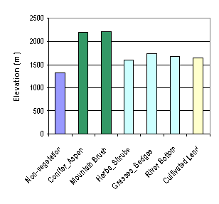
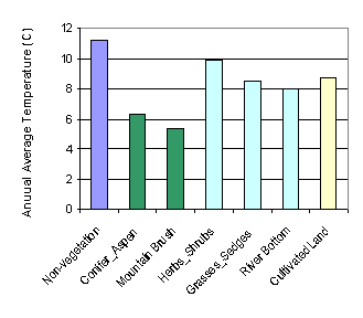
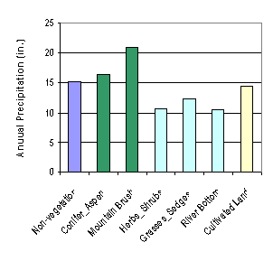
Figure 11. Compare zonal means of elevation and climate conditions in different vegetation zones

5. DISCUSSION AND CONCLUSIONS

In this term project, only elevation was considered when interpolating climate data. In fact, other factors can also affect climate conditions. For example, slope and aspect can affect radiation received and thus temperature. Considering more factors needs to use complicated climate models and their data must be available. In addition, only elevation and climate conditions were considered to classify vegetation distribution. But vegetation distributions are also affected by other factors such as soil types. All these will be considered in future work.

Besides, I tried to divide the chosen weather stations into two groups, so that on group could be used for interpolation and the other for testing the results of interpolation. But I found that different division of groups would produce different rates by which annual average temperature and annual precipitation change with elevation, and thus different interpolation results. So it is hard to say how reliable this testing method itself is. So I didn’t do it in this term project, and left it as future work. In the future work, I will explore how to divide the sample data into two groups is reliable, and check the validation of interpolation with ‘out of sample testing’ and by comparing interpolation with other models.

For this term project, temporary conclusions are:

(1) GIS is a convenient tool to get area data from point data, especially when topography is complicated.

(2) Some parameters change with elevation, e.g., lapse rate of annual average temperature is about 6 °C/km in Utah, though it may be uncertain when elevation is out of data range. Elevation should be included when they are interpolated.

(3) Tension Spline method may be more suitable than Regularized Spline method to interpolate point data of climate conditions into grid data.

(4) Herbs-shrubs and conifer-aspen account for more than 70% of Utah area.

(5) With only elevation, annual average temperature and annual precipitation considered, vegetation in Utah could be roughly divided into three classes: conifer-aspen and mountain brush averagely are located at higher elevation with lower annual average temperature and more annual precipitation, while vegetation of herbs-shrubs, grasses-sedges, and river bottom is contrary. Cultivated lands are specially located at lower elevation with higher temperature and more precipitation.

6. ACKNOWLEDGE

I would like to acknowledge to Dr. David Tarboton for his help in this term project and during the study of the course. I also appreciate Mr. Shujun Li for his offering some data and help for GIS problems in the project.

7. REFERENCE

Michael Zeiler, 1999, Modeling our World – the ESRI guide to Geodatabase design, ESRI Press,