Prediction of Channel Geometry from DEM-Derived
Channel Slope
Jason Thompson
CEE 6440 GIS in Water Resources
Introduction
Objectives
Introduction
The
Objectives
This study had three primary objectives. The first objective was to use tools
available in ArcMap to derive channel slope for the
Manning’s Equation
Channel slope and channel geometry are related through Manning’s Equation. This equation is a widely used empirical equation used for estimating discharge from channel characteristics. Manning’s Equation is given below:

In this equation, Q is equal to the discharge (cfs); Cu is a conversion factor equal to 1.486 when using ES units; n is the Manning’s roughness factor; A is the wetted cross-sectional area (ft2); Rh is the hydraulic radius (ft), equal to the wetted cross-sectional area divided by the wetted perimeter; and S0 is equal to the energy slope, or for uniform flow S0 can be approximated by the slope of the channel bottom. For the purposes of this study, channel geometry is represented by the term ARh2/3 in Manning’s Equation. This term is equivalent to the cross-sectional area raised to the 5/3 power divided by the wetted perimeter raised to the 2/3 power. Wetted perimeter is the length of the channel in cross-section view in contact with the water in the channel. The geometry features of interest are depicted in Figure 3. According to Manning’s Equation, the calculation of channel geometry requires the discharge (Q), Manning’s roughness (n), and the channel slope (S0):

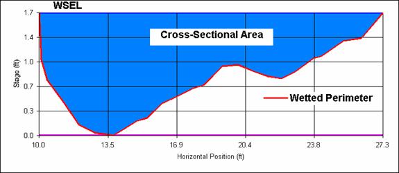
Figure 3. Description of channel geometry
Determination of Channel Slope
In order to
predict channel geometry, the slope of the channel must be calculated. Assuming this value has not been measured in
the field, some other means of obtaining this value would need to be
identified. The possibility exists of
using slope derived from a DEM for such a purpose. However, it is obvious that a DEM with a cell
size of 900-m2 could not be used for effectively calculating channel
slope except for the case of a very large river. While it may not be feasible to estimate
channel slope for smaller streams, it is still possible to accurately estimate
valley slope. Valley slope refers to the
slope of the valley in which the stream flows.
Because valleys are larger features than channels, their slope should be
able to be predicted from a 30-m DEM.
Channel slope can be related to valley slope through channel
sinuosity. Channel sinuosity is defined
as the ratio of the length of the stream to the length of the valley. Sinuosity can also be described as the ratio
of the valley slope to the channel slope (Rosgen 1994). Based on these relationships, the following
equation can be used to calculate the channel slope:

Before any
of the above factors could be calculated, the hydrography data for the Upper
Virgin River Watershed (HUC 15010008) was obtained from the USGS National
Hydrography Dataset (http://nhd.usgs.gov/). All the data used in this study was projected
in UTM Zone 12 NAD83. Then the
The valley length for each
segment was assumed to be equivalent to the straight-line length of each
segment. This approximation is often
made when calculating sinuosity. The
length of each segment was calculated using the following procedure: (1) a line Feature Class was created in a
Feature Dataset in ArcCatalog; (2) the line Feature Class was added into
ArcMap, and the line was constructed along the length of a segment using the
ArcMap Editor; (3) upon completion of the editing, the length of the line was
automatically calculated. This procedure
was repeated for all 29 segments. Each line
length was then added into the attribute table of its corresponding
segment. Figure 5 (in Appendix) shows each of the
distinct lines created along the length of each segment for the
Once values of stream length and
valley length were calculated for each segment, then the sinuosity of each
segment was easily calculated. These
calculations were performed in Excel.
Once these calculations were done, the sinuosity values for each segment
were added to the appropriate segment attribute table. The segments were merged together and a map
was produced showing sinuosity values associated with 1-km segments of the
The final component required for the calculation of the channel slope was the valley slope. The first step was the calculation of slope (%) in a raster format (grid cell size of 900-m2) from a DEM using Spatial Analyst in ArcMap. The 30-m DEM was obtained from the USGS National Elevation Dataset (http://edcnts12.cr.usgs.gov/ned/default.htm). Before the slope calculation, the pits in the DEM were filled using TauDEM. Three different approaches were used for the estimation of valley slope. Different approaches were used in order to compare varying methodologies in an attempt to identify the most useful approach and evaluate the resulting values for valley slope. The first approach was to estimate valley slope as simply elevation change divided by the change in distance for each segment. Elevations were obtained directly from the DEM at the beginning and end points of each segment using the identify tool in ArcMap. Because the distance between those segment endpoints was previously determined, the slope could be calculated along the segment. This method was referred to as the linear slope method, and provided a simple means of estimating valley slope. The values of slope were then added to the attribute table for each segment. Figure 7 (in Appendix) shows the slope values for each stream segment obtained using this method.
The second approach used for
estimating valley slope involved calculating the average slope within a buffer
established around the stream. This
approach was chosen because it was initially thought that the slope within the
stream buffer would provide an adequate representation of the stream valley slope. While the first approach approximated slope
based on elevation values about 1 km apart, this approach estimated average
slope based on numerous slope values in an area adjacent to the stream. Initially, the ArcMap Buffer Wizard was used
to construct a 30-m buffer around the
The channel slopes resulting from the
linear slope, 30-m buffer, and 15-m buffer estimation methods are presented graphically
in Figure
10 below. This chart shows
that the two buffer methods predicted fairly similar channel slopes, but greater
values than the linear slope method.
There does not appear to be a distinct trend between slope and segment
location with the linear slope method.
With the two buffer methods, there does appear to be a general trend of
increasing slope with segment location upstream to segment 22-23.
Besides calculating channel slope
from valley slope using sinuosity, channel slope was also estimated directly
from the slope raster produced from the DEM using Spatial Analyst. The identify tool in ArcMap was used to
determine slope values at several locations on the
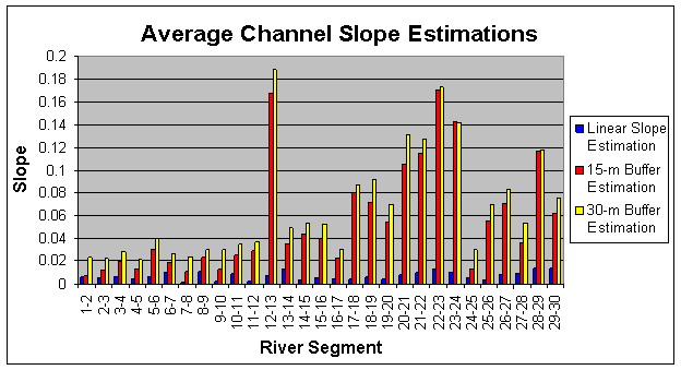
Figure 10. Estimations of channel slope from three
methods
Predictions of Channel Geometry
As mentioned above, cross-sections
were established on the
n = (nb + n1 + n2 + n3
+ n4)m, where nb is the base value of n, n1 is
a correction for surface irregularities, n2 is a correction for
cross-section size and shape, n3 is a correction for obstructions, n4
is a correction for vegetation, and m is a correction for channel
meandering. The final parameter required
is channel slope, which was estimated using the four different methods
discussed above. The results of the
channel geometry calculations are presented in Figure 12
below.
Table 1. Manning’s roughness factor for each
cross-section
|
X-SEC |
n |
nb |
n1 |
n2 |
n3 |
n4 |
m |
|
1 |
0.02 |
0.02 |
0 |
0 |
0 |
0 |
1 |
|
2 |
0.02 |
0.02 |
0 |
0 |
0 |
0 |
1 |
|
3 |
0.031 |
0.03 |
0.001 |
0 |
0 |
0 |
1 |
|
4 |
0.031 |
0.03 |
0.001 |
0 |
0 |
0 |
1 |
|
5 |
0.031 |
0.03 |
0.001 |
0 |
0 |
0 |
1 |
|
6 |
0.031 |
0.03 |
0.001 |
0 |
0 |
0 |
1 |
|
7 |
0.03565 |
0.03 |
0.001 |
0 |
0 |
0 |
1.15 |
|
8 |
0.03565 |
0.03 |
0.001 |
0 |
0 |
0 |
1.15 |
|
9 |
0.031 |
0.03 |
0.001 |
0 |
0 |
0 |
1 |
|
10 |
0.031 |
0.03 |
0.001 |
0 |
0 |
0 |
1 |
|
11 |
0.03565 |
0.03 |
0.001 |
0 |
0 |
0 |
1.15 |
|
12 |
0.03565 |
0.03 |
0.001 |
0 |
0 |
0 |
1.15 |
|
13 |
0.031 |
0.03 |
0.001 |
0 |
0 |
0 |
1 |
|
14 |
0.031 |
0.03 |
0.001 |
0 |
0 |
0 |
1 |
|
15 |
0.031 |
0.03 |
0.001 |
0 |
0 |
0 |
1 |
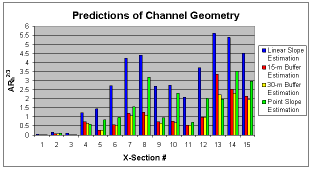
Figure 12. Channel geometry predictions for each
cross-section
Figure 12 shows
that in general, the linear slope method predicted the highest values of
channel geometry for each cross-section, followed by the point slope
method. The two buffer methods typically
predicted the lowest values. With all
four methods, channel geometry values were relatively small for the first three
cross-sections with an increase between cross-sections 4 and 8. Each of the methods, with the exception of
the point slope method, predicted fairly similar geometry values for
cross-sections 9 through 12, but differences existed between the methods. For the linear slope method and the two
buffer methods, the highest geometry values predicted for all the
cross-sections occurred for cross-sections 13 through 15. The point slope method was more
variable.
Comparing
Predicted and Measured Channel Geometry
The final
objective of this study was to compare the predicted values of channel geometry
with the values measured at each of the cross-sections. As stated previously, distance-elevation data
were surveyed along each cross-section.
However, this data needed to be converted to the form of channel
geometry used in this study (ARh2/3). In order to derive cross-sectional area and
hydraulic radius from the survey data, the program WinXSPRO, developed by the
USDA Forest Service, was used. One of
the operations available with WinXSPRO is the conversion of distance-elevation
pairs into channel cross-sectional area and wetted perimeter, from which the
hydraulic radius can be calculated. Figures
13, 14, 15, and 16 (in Appendix)
compare the measured channel geometry values with those predicted by the linear
slope, point slope, 30-m buffer, and 15-m buffer methods, respectively. Figure 17 below summarizes the predicted
and measured geometry values. This
figure shows that in general, the measured geometry values were much greater
than the predicted values. Of the four
prediction methods, the linear slope method produced geometry results most
similar to the measured values, followed by the point slope method. The two buffer methods did not predict
geometry well relative to the measured values.
Figure 18 below shows the differences in percent between the
measured and predicted geometry values.
The information in this figure reaffirms the above observation that the
linear slope method produced results most similar to the measured values. The two buffer methods produced very similar
results, with the 15-m buffer method predicting only slightly better in
general. This result indicates that
changing the buffer size from 30-m to 15-m did not markedly improve the
prediction power of the buffer method. It
is interesting to note from Figure 17 that although the linear slope
method predicted lower geometry values than those measured, there appears to be
a similar trend between the values. In a
further attempt to investigate data trends, Figure 19 was
produced. In this figure, the
multiplicative factor on the y-axis was obtained by simply dividing the
measured geometry value by the predicted value for each of the methods. The differences in Figure 19 between
the measured and predicted values are initially very high for all four methods
but then tend to decrease with upstream cross-section. As expected, both buffer methods exhibit very
similar trends in this figure. The point
slope method displays a similar trend to the buffer methods, but in a less
pronounced, more dampened manner. This
figure also shows that the linear slope method and the measured values do
exhibit a similar trend, particularly upstream of and including cross-section
3. At these cross-sections, the
multiplicative factor maintains a fairly constant value, indicating a
relatively uniform relationship. The
relationship between the other methods’ predictions and the measured values
appears to be much more variable.
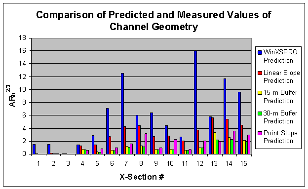
Figure 17.
Geometry summary comparison
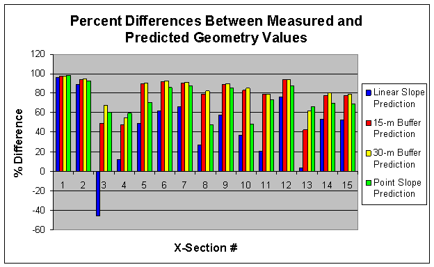
Figure 18.
Differences (%) between measured and predicted geometry
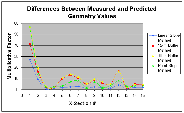
Figure 19. Differences between measured and predicted
geometry
Conclusions
Based on the above study, several
conclusions can be drawn regarding the applicability of predicting channel
geometry from Manning’s Equation, with the channel slope in the aforementioned
equation derived from a DEM. In this
particular study, none of the four techniques used for estimating channel slope
consistently produced channel geometry values similar to the values measured at
each cross-section. Of the techniques
used, the linear slope method predicted geometry most accurately relative to
the measured values. Geometry values
predicted by the linear slope method and the measured values also exhibited a
very similar trend based on cross-section location. Using slope values directly from the slope
raster at each cross-section location did not prove to be a reliable method for
estimating channel slope at that location.
Both the 30-m and the 15-m buffer methods predicted similar geometry
values, but underestimated geometry relative to the measured values. The inaccuracy of these buffer methods was
most likely due to the topography characteristics adjacent to the
1.
Cowan, W.L. 1956. Estimating hydraulic roughness
coefficients. Agricultural
Engineering 37(7): 473-475.
2. Rosgen, D.L. 1994.
A classification of natural rivers.
Catena 22(1994): 169-199.
Appendix
Figures 1-16
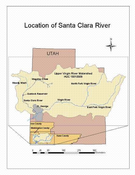
Figure 1. Map
of the
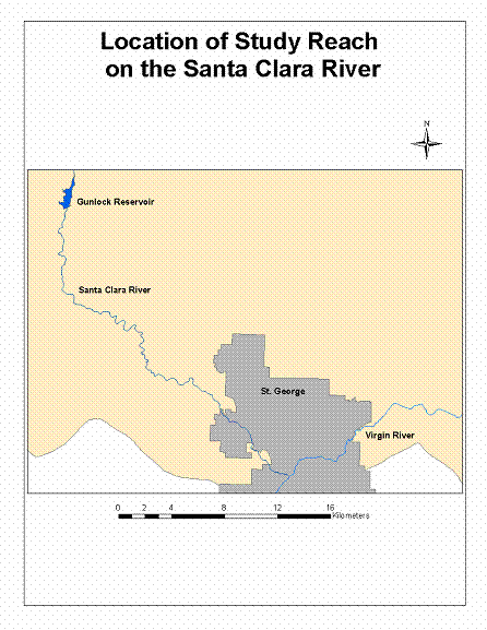
Figure 2. Map
showing the
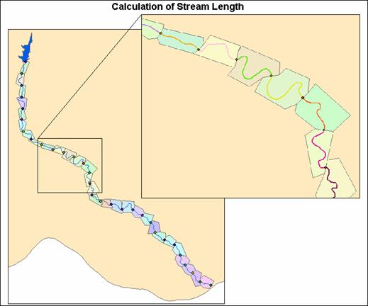
Figure 4.
Polygons and stream reaches for the stream length calculation
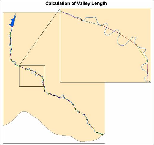
Figure 5. Lines created for the calculation of valley length
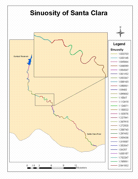
Figure 6. Map of the sinuosity of
the Santa Clara
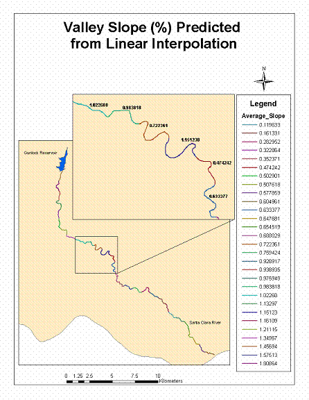
Figure 7. Map of
valley slope from linear slope method
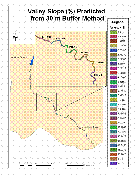
Figure 8. Map
of valley slope from 30-m buffer method
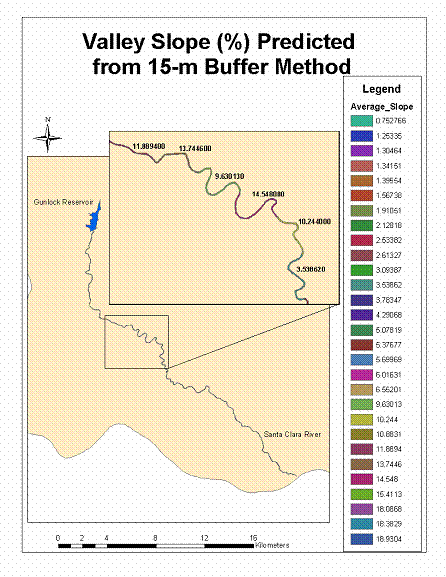
Figure 9. Map
of valley slope from 15-m buffer method
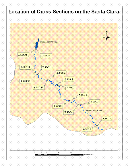
Figure 11.
Cross-sections on the
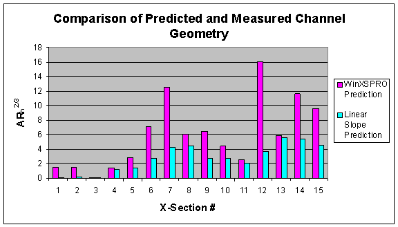
Figure 13.
Geometry: measured vs. predicted
from linear slope method
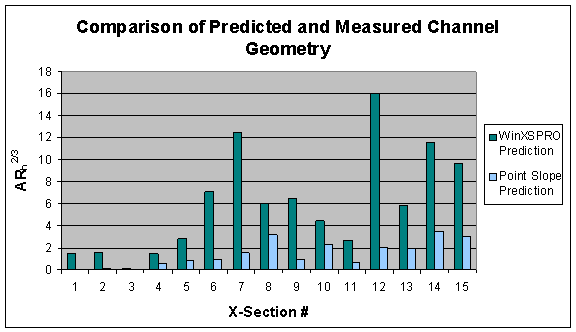
Figure 14.
Geometry: measured vs. predicted
from point slope method
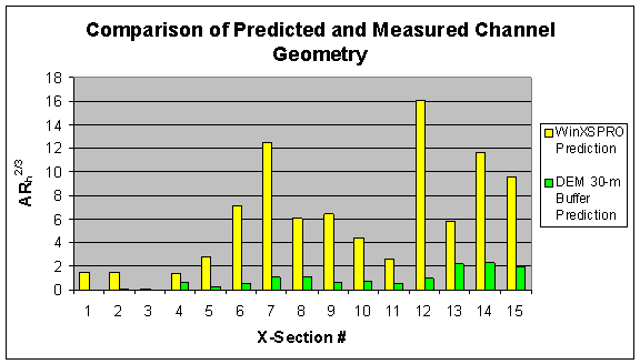
Figure 15.
Geometry: measured vs. predicted
from 30-m buffer method
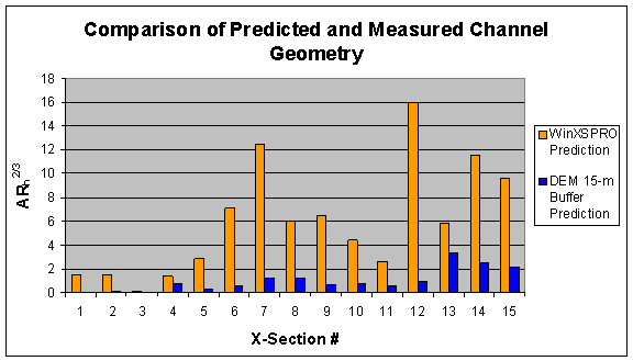
Figure 16.
Geometry: measured vs. predicted
from 15-m buffer method