Background of the Project
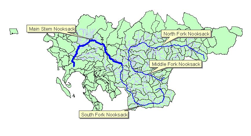
The Nooksack River watershed is located in northwestern Washington, encompassing Whatcom County and part of Skagit County, and reaching northward into British Columbia. The watershed is large, covering about 1,250 square miles with more than 1,000 stream and river miles. The Nooksack's headwaters lie within National Park and National Forest boundaries. Much of the middle watershed is managed for timber production by private timber companies and the Washington State Department of Natural Resources. River valleys and the lower watershed support agriculture and rapidly developing residential areas.

Diverse habitats throughout the Nooksack watershed support a variety of fish and wildlife. The upper watershed is important to bull trout, grizzly bear, and bobcat. The middle watershed provides habitat for wintering bald eagles, deer, elk, and hawks. The lower watershed hosts shorebirds, waterfowl, herons, snowy owls, gyrfalcons, and peregrine falcons. The watershed's rivers and streams are vital fish habitat for chinook, coho, chum, sockeye, pink, and steelhead salmon, as well as both resident and sea-run cutthroat trout.

Goal of the Project
Numeric studies, aimed to better understand natural processes, to be able to predict them in the future and improve current situation, have been conducted on the watershed for years. Last Spring - Autumn an  Institute for Natural Systems Engineering (INSE, USU)  field crew collected a set of cross-sectional data along the mainstem Nooksack River. The data included velocities, depths and discharges for each cell along a cross-section. Within this project these data along with some others are going to be used to calculate travel times for the reaches along the mainstem and total travel times for a range of discharges. Such information can be used later for answering some questions related to fish habitat, water quality, etc.

Data used
The data used for this project included EPA River Reach File (RF3), USGS 10 m DEM, Digital Raster Graphic (7.5' quads) which had to be projected since the data were in Datum NAD 27, so it had to be adjusted to the rest of the data which were in Datum NAD 83. Adjustments were performed using program CORPSCON which, given coordinates of the upper left corner of the quad in NAD 27, calculates new coordinates  in NAD 83.

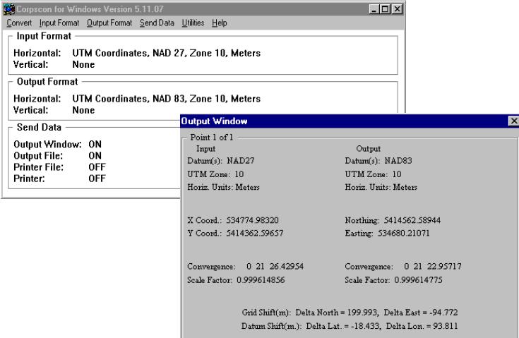
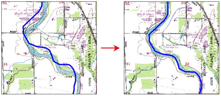
The new coordinates are then saved in the tiff-world file (*.tfw) which places the image in the right place. AND HERE IS THE RESULT!

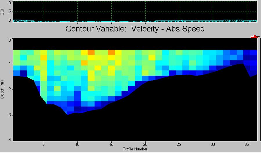
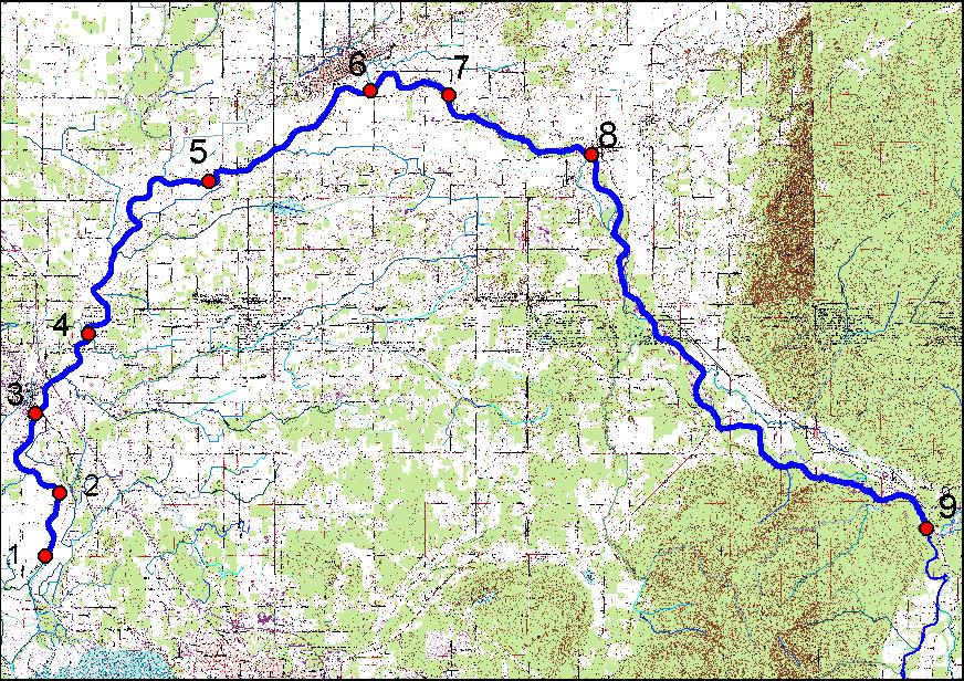
Field data included measurements of 9 cross-sections along the mainstem on September 14, 2000. The data were collected using Acoustic Doppler Profiler (ADP) and analyzed using River Surveyor Software which as an output produces velocities, depths, discharges, directionS of flows, etc., for each cell along cross-section.
 

These data then imported into R2CROSS program which uses cross-sectional data for one discharge and slope of the reach and applying Manning's equation predicts average velocities and discharges for the range of Q up and down from the given Q through fixed increments of depths.

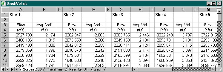
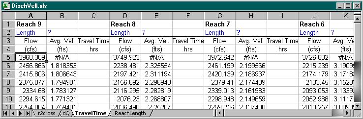
That output is used for calculation of Travel Times within Excel. In the next step we set control flows for which we are looking for the relationship TT vs. Q. There is USGS gaging station right next to one of the sites (Site 9) so, we use a set of flows for this site as a reference flows and related the flows for remaining sites to these through dQ (the difference in flows between the sites). Within this project, since the data for only one flow were available, only one dQ for each section was used for the whole range of discharges. As the information becomes available later (we collect more data at different discharges), obviously, it is easy to incorporate it into the analysis. For calculated set of discharges for a range of flows for each site we interpolate velocities from the "r2cross" spreadsheet (previous image) and the only missing parameter for calculation of the travel times is the length of the stream.

We can simply divide the stream into reaches and calculate their length manually but then every time we change our criteria for dividing the stream into reaches or join/ divide the reaches into smaller sections we would have to go and repeat the  procedure again. We prefer this to be a little more automatic that is why we use ArcView to produce the lengths.

The first step is to place our cross-sections on proper places. It was done manually since no more precise information then visual was available (there were no GPS measurements made). In this case it works perfectly fine since after dividing the stream into reaches we are going to say that each reach is represented by the average velocity from corresponding cross-section, thus it is not really important if the cross-section is +/- 20 m away. Besides, using quads the position can be found quite easily.

The next step is to define the reaches. As it was noted earlier, the criteria for braking the stream into reaches can be different: it depends on what question we are trying to answer. As an example, I used slope as a criteria, so every reach represents an area of equal slope. Yellow dots are the reachbreaks.

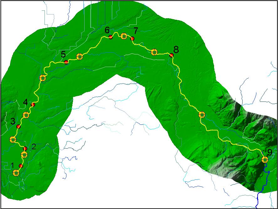
Then, using Network Analyst we determine the best route between the reachbreaks (yellow line on the image), which gives us length between the points. Selecting everything in the attribute table and choosing a particular cell in the Excel Spreadsheet

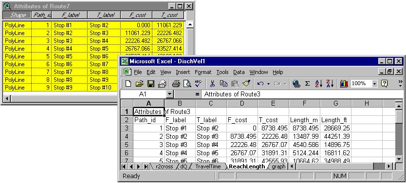
we use Dynamic Data Exchange link (DDE) to update the spreadsheet.

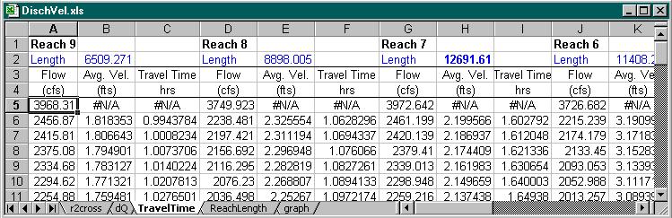
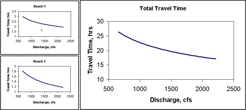
This last step automatically gives us  plots of Travel Times vs. Discharges for each reach and for the whole mainstem for a range of discharges.

Conclusions
As a result of this project an interactive system was built which allows us to determine the relationships between Travel Times and Flows for different conditions without the necessity to perform the whole procedure every time we change a  parameter. We can update hydrologic and hydraulic data, change reach lengths and the system will provide results with minimum efforts.

Acknowledgments
- people working for INSE who helped me get and analyze the data;
- Mark Winkelaar who helped me a lot in implementing this idea.

References