TauDEM, Terrain analysis using Digital Elevation Models

David G. Tarboton                                                        July 18, 2001
Utah State University
8200 Old Main Hill
Logan, UT 84322-8200
USA
http://www.engineering.usu.edu/dtarb/
email:  dtarb@cc.usu.edu

TauDEM is a still somewhat experimental effort to develop a graphical user interface version of my programs that have been available in command line version for several years.  This program is Copyright (C) 2001  David Tarboton, Utah State University.  This program is distributed for free in the hope that it will be useful, but WITHOUT ANY WARRANTY; without even the implied warranty of MERCHANTABILITY or FITNESS FOR A PARTICULAR PURPOSE.

Installation

Download taudem.exe.  The installation package and software was built for Windows 98.

The programs and what they do.

Click on commands and buttons below to go to the help for them.

Startup Dialog Box

• Load DEM Grid: To work with a new DEM grid file. Grid file can be any of the following formats, ESRI, ASCII or TMDL toolkit binary grids.
• Load existing (previously saved) project: To open an existing Taudem Project (*.tdp) file.

Button Bar

The tools in the button bar are used to navigate within the project, and to execute functions.

These buttons start a new TauDEM project, open an exsiting project from a *.tdp file or save the current project in a *.tdp file.

Zoom to full extents

This button scales the map window to the extents of the current project.

Zoom in

This tool allows the user to view a smaller region of the map in greater depth. Click in the map window on the region of study. When the zoom in feature is selected, a left mouse click will zoom in, and a right mouse click will zoom out. To zoom to a specific area, left click and drag the mouse to enclose the area. The view will then zoom to those extents.

Zoom out

When selected, this tool will show more of the map in less detail. A left click will zoom out; a right click will reverse the process.

Zoom to previous extents

This will get back the last position of the map on the map window. It can be used along with Zoom-in and Zoom-out to get the desired view of the map. When the user zooms in/out mistakenly, he can use this tool to get back at his previous view.

Pan

This tool moves the portion of the map on display in the map window. Click on a region of the map and drag the mouse; dragging to the left will display the map to the right, and vice versa.

Select Cursor

This tool is used to select grid cells or graphical objects.  At present this is used for the selection of outlet points.

Add layer

This button allows users to add a new layer in the project. At present bitmap images and shape files are the only data formats supported.  Data layers added should have consistent geographic projections.

Remove Selected Layer

This tool will remove the selected layer from the project.  Layers may be selected by clicking in the layer list window.

Clear all layers

To remove all the layers from the map window.

Layer Order arrows

These arrows control the order in which layers are displayed.  Layers at the top in the legend are displayed on top of lower layers.

Menu Bar

File menu options

• Prepare Connected Reach Network From Shape File: This launches a 'Network Builder' form that will take any polyline shape file and build a connected reach network file.
• This Select Existing Connected Reach Network File: This MUST have as input a reach file created previously by the 'Network Builder'.

DEM menu options

• Do all preprocessing: This runs the commands given below in sequence
• Convert connected reach network to forced flow direction grid: This takes as input a network river reach file from the network builder and outputs a grid of flow directions along the rivers to enforce drainage along delineated river channels.  These flow directions are in a file with suffix 'fdr' and are used by Flood if the option to use them under River Network and Watersheds/Method Options is set.
• Fill pits and nondraining hollows: This takes as input an elevation data grid and outputs a grid file 'fel' with pits filled, using the flooding algorithm.  The river flow enforcement direction grid is an optional input, and if input, pits will be filled consistent with drainage along existing streams.
• Compute D8 flow directions: This takes as input pit filled elevation data file 'fel' and outputs D8 flow directions 'p' and slopes 'sd8' for each grid cell. The following coding is used for direction of flow from a pixel to ONE of its eight neighbors:
  4 3 2
  5    1
  6 7 8
  In flat areas flow directions are assigned away from higher ground and towards lower ground using the method of Garbrecht and Martz (1997).  The river flow enforcement direction grid is an optional input, and if input, directions will be set consistent with drainage along existing streams.
• Compute Dinf flow directions: The Dinf approach assigns a flow direction based on steepest slope on a triangular facet (Tarboton, 1997). This is saved as an angle 'ang' in radians anti-clockwise from east. In flat areas the D8 flow directions are converted to angles and used.
• Compute drainage area by D8 method: This takes as input a D8 flow directions file 'p' and outputs the contributing area. The result is the number of grid cells draining through each grid cell.  By default the program checks for edge contamination.  The edge contamination checking may be overridden with an option in the River Network and Watersheds/Method Options form.
• Compute specific catchment area by Dinf method: This takes as input a Dinf angle file 'ang' and outputs the specific catchment area. Specific catchment area is defined as contributing area per unit contour length.  Here the contour length is taken as the grid cell size.  The result has length units the same as grid cell size.  By default the program checks for edge contamination.  The edge contamination checking may be overridden with an option in the River Network and Watersheds/Method Options form.
• Compute grid network order, Upslope total flow length, Upslope longest flow length: This takes as input a D8 flow directions file 'p' and outputs three grid files:
  'plen'  Each grid cell contains the path length from the furthest cell that drains to each cell.
  'tlen'  Each grid cell contains the total length of all paths draining to each cell.
  'gord'  Each grid cell contains the Strahler order associated with that cell for a flow network defined using the D8 flow directions and including each grid cell.  Strahler order is defined as follows. Cells that don't have any other grid cells draining in to them are order 1.  When two (or more) flow paths of different order join the order of the downstream flow path is the order of the highest incoming flow path.  When two (or more) flow paths of equal order join the downstream flow path is increased by 1.  Algorithmically this is implemented as:
  Order = Max(Highest incoming flow path order, Second highest incoming flow path order + 1)
  These outputs are used by netsetup in some of the options for mapping channel networks.

River Networks and Watersheds menu options

• Do all watershed and network delineation steps: This runs the commands given below in the correct sequence.
• Specify outlets:  Brings up a form that allows you to click on the map to identify outlets.
• Set or Change Method Options...: This brings up a form to toggle various method options and control network delineation methods.
• River Network Raster (Full):  This uses the network delineation parameters to define a grid of the river network, useful for identifying outlets.  Valid outlet points are only those on the 'src' grid produced here.
• River Network Raster (Upstream of Outlets):  This uses the network delineation parameters to define a grid of the river network, upstream of the outlets.  This is necessary for the creation of networks and subwatersheds.
• Drop Analysis: This brings up a table of stream drops useful for identifying the correct channel network identification threshold.
• Create Network and Sub-Watersheds:  This converts the grid of river network cells into a shapefile with attributes for each reach.  Local watersheds draining to each reach are also delineated as a grid and shape file.
• Compute distance to streams: This computes a grid where the value in each grid cell location is the distance along the flow path to the nearest stream (as delineated by the Create Network and Sub-Watersheds function).

If drop analysis is checked, then the threshold is searched between the lowest and highest values given, using the number of steps given on a log scale.  For the science behind the drop analysis see Tarboton et al. (1991, 1992), Tarboton and Ames (2001).  The smallest threshold in the set searched with absolute value of the t statistic less than 2 is selected.  This is done automatically during the River Network Raster (Upstream of Outlets) step.  The threshold selected is saved in the threshold variable so may be inspected afterwards by viewing the options window.

The "Drop Analysis" command displays a table showing the information used in the drop analysis, as follows

The columns are:
Threshold:  The threshold used in the network delineation algorithm.
Dd:  The drainage density (inverse length units - typically m) of the resulting network.
n1:  Number of first order streams (Strahler ordering) in network with specified threshold.
nh:  Number of higher order streams (Sequential segments of the same order are counted as one Strahler stream) in network with specified threshold.
md1:  Mean drop (elevation difference between start and end) of first order streams.
mdh:  Mean drop of higher order streams.
sd1:  Standard deviation of first order stream drops.
sdh:  Standard deviation of higher order stream drops.
t: Students t statistic for the difference between the first order and higher order mean stream drops.

The procedure suggested in Tarboton et al. (1991, 1992) and Tarboton and Ames (2001) is to select the smallest threshold for which the absolute value of the t statistic is less than 2.  This selects the highest resolution network consistent with the "constant drop law".  In the display above the threshold of 50 would be selected.  It is worthwhile to view the drop analysis because the threshold steps are sometimes quite coarse, so the user may want to use the Specify Method Options command to change the number of intervals and lowest and highest values used in the search.  Also it can occur that a large threshold is "correct" but a small threshold results in second or higher order streams also extending into the region that should not be streams.  If these dominate the sample the following sequence of t statistics might result:
<2, <2, <2, >2, >2, <2, <2, ...
The automatic procedure in these cases would pick the lowest threshold, but it is probably better (and this is admittedly subjective, unfortunately) to pick the 6th threshold.  In making this judgement I feel that it is best to consider many things, like sample sizes (is the t statistic robust), the visual impression in comparison to contour crenulations, and the drainage density that would result from a Slope versus Area plot as discussed in Tarboton et al., (1991, 1992).  The automated procedure is therefore not foolproof and some degree of judgement and subjectivity is required.
 

Model Setup menu options

Topmodel Setup

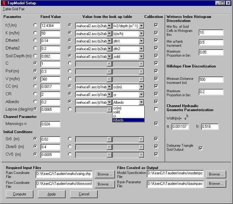
The variables under 'Parameter' and 'Initial Conditions' can be assigned a fixed value or be set to be read from a look-up table associated with a variable classification grid by selecting the radio buttons. If the option of look-up table is chosen the user has to load the appropriate grid-table pair. Also, the user has to assign each variable the corresponding grid-table pair and the field in the table, from which the value has to be read. Combo boxes under 'Value from the look up table' help in making the selections. The lookup table should be a comma delimited text file with one header row and first column giving the key to associate parameters in the table with classification values in the corresponding grid.  Following is an example of a lookup table:

Soil_type_number,f (m^-1),k(m/h),dth1,dth2,soil name,depth(metres)
1,1.82,0.0026,0.084,0.131,ANS,1.1
2,2,0.0054,0.123,0.106,C1,1
3,1,1,0.1,0.1,N/A,0.72
4,3.33,0.001,0.087,0.158,KR,0.6
5,1.92,0.03,0.111,0.26,MT,1.04
6,1,1,0.1,0.1,N/A,0.72
7,1,1,0.1,0.1,N/A,0.9
8,2.67,0.001,0.099,0.138,PBuH,0.75
9,2.22,0.0004,0.117,0.107,WA/WAH,0.9
10,3.33,0.0066,0.113,0.16,WF/WO,0.6
...

The checkboxes on the right (under calibration) control whether resulting model element parameters can be calibrated by multiplying by a factor to retain the spatial patterns provided through the GIS information in the classification grid.

Rain Coordinate file and Flow Coordinate file are the files required by the module to generate the output files, that are Model Specification file and Basin Parameter file. Rain Coordinate file is a shape file (extension '.shp') that contains the raingage point locations.  The flow coordinate file has not been implemented yet.

Topmodel uses a histogram discretization of the topographic wetness index (ln(a/S) from the wetness index function above).  The parameters in the right pane control the bin size associated with this histogram.  Topmodel also uses a histogram discretization of overland flow distances to channels (computed with the distance to stream function above).  The parameters in the right pane control the bin size associated with this histogram.

The kinematic wave flow routing part of TOPNET needs channel widths.  These are estimated based on geomorphology using the drainage area and the hydraulic geometry function with parameters in the right pane.

Topmodel estimates the rainfall input to each model element using weights based upon delauney triangles.  The delayney triangle check box controls the output of a grid depicting these triangles so that they may be displayed.

Background on working with Digital Elevation Models

Pits in digital elevation data are defined as grid elements or sets of grid elements surrounded by higher terrain that, in terms of the DEM, do not drain. These are rare in natural topography and generally assumed to be artifacts arising due to the discrete nature and data errors in the preparation of the DEM. They are eliminated here using a 'flooding' approach. This raises the elevation of each pit grid cell within the DEM to the elevation of the lowest pour point on the perimeter of the pit . Slopes and Flow Directions

Working with grid DEMs slope may be computed as the difference in elevation between two adjacent cells divided by the distance between them. In dealing with flow this is usually done in a forward downwards direction. The slope associated with a cell is the slope from the cell to a downslope neighbor. This makes sense because it is where water will go. Radiation computations sometimes use slope based upon central finite difference methods. The earliest and simplest method for specifying flow directions is to assign flow from each grid cell to one of its eight neighbors, either adjacent or diagonally, in the direction with steepest downward slope. This method, designated D8 (8 flow directions), was introduced by O'Callaghan and Mark (1984) and has been widely used. The D8 approach has disadvantages arising from the discretization of flow into only one of eight possible directions, separated by 45^odeg; . These have motivated the development of other methods comprising multiple flow direction methods , random direction methods and grid flow tube methods . Tarboton (1997) discusses the relative merits of these.

In the D¥ method, the flow direction angle measured counter clockwise from east is represented as a continuous quantity between 0 and 2p. This angle is determined as the direction of the steepest downward slope on the eight triangular facets formed in a 3 x 3 grid cell window centered on the grid cell of interest as illustrated in figure 1. A block-centered representation is used with each elevation value taken to represent the elevation of the center of the corresponding grid cell. Eight planar triangular facets are formed between each grid cell and its eight neighbors. Each of these has a downslope vector which when drawn outwards from the center may be at an angle that lies within or outside the 45^o (p/4 radian) angle range of the facet at the center point. If the slope vector angle is within the facet angle, it represents the steepest flow direction on that facet. If the slope vector angle is outside a facet, the steepest flow direction associated with that facet is taken along the steepest edge. The slope and flow direction associated with the grid cell is taken as the magnitude and direction of the steepest downslope vector from all eight facets. This is implemented using equations given in Tarboton (1997).

In the case where no slope vectors are positive (downslope), the flow direction is set using the method of Garbrecht and Martz (1997) for the determination of flow across flat areas. This makes flat areas drain away from high ground and towards low ground. The D¥ method is preferred for the computation of flow directions on hillslopes where D8 grid bias is significant in the calculation of specific catchment area. D8 is still used for the definition of channel networks because we can not (have not yet learned to) work with channel networks that bifurcate in a downwards direction.

Contributing Area

The contributing area programs check for edge contamination .  This is defined as the possibility that a contributing area value may be underestimated due to grid cells outside of the domain not being counted.  This occurs when drainage is inwards from the boundaries or areas with no data values for elevation.  The algorithm recognizes this and reports no data for the contributing area.  It is common to see streaks of no data values extending inwards from boundaries along flow paths that enter the domain at a boundary.  This is the desired effect and indicates that contributing area for these grid cells is unknown due to it being dependent on terrain outside of the domain of data available.  The edge contamination checking may be overridden with an option in the River Network and Watersheds/Method Options form in cases where you know this is not an issue or want to ignore these problems, if for example the DEM has been clipped along a watershed outline.

Channel Networks

Data formats

• ncols - number of columns in the data set.
• nrows - number of rows in the data set.
• xllcenter or xllcorner - x-coordinate of the center or lower-left corner of the lower-left cell.
• yllcenter or yllcorner - y-coordinate of the center or lower-left corner of the lower-left cell.
• cellsize - cell size for the data set.
• nodata_value - value in the file assigned to cells whose value is unknown. This keyword and value is optional. The nodata_value defaults to -9999.

ncols 480
nrows 450
xllcorner 378923
yllcorner 4072345
cellsize 30
nodata_value -32768
43 3 45 7 3 56 2 5 23 65 34 6 32 etc
35 45 65 34 2 6 78 4 38 44 89 3 2 7 etc
etc

Grid naming convention.

The following default naming convention is suggested and used by the software.  Any file names may be used with interactive input, but I suggest sticking to this convention to avoid confusion.  File names are:
nnnnsss[.asc]
nnnn comprises the name of the dataset. Maximum length is operating system dependent.
sss comprises the suffix used to designate the data type as follows:

no suffix.	Elevation data.
fel	Pit filled elevation data.		produced by Fill pits and nondraining hollows
p	D8 drainage directions.		produced by D8 flow directions
sd8	D8 slopes.		produced by D8 flow directions
ad8	D8 contributing area’s, units are number of grid cells.		produced by D8 drainage area
slp	Dinf slopes.		produced by Dinf flow directions
ang	Dinf flow directions.		produced by Dinf flow directions
sca	Dinf contributing area, units are specific catchment area, i.e. number of grid cells times cell size.		produced by Dinf drainage area
plen	Longest path length to each grid point along D8 directions.		produced by Grid network order, Upslope total flow length, Upslope longest path length function
tlen	Total path length to each grid point along D8 directions.		produced by Grid network order, Upslope total flow length, Upslope longest path length function
gord	Strahler order for grid network defined from D8 flow directions.		produced by Grid network order, Upslope total flow length, Upslope longest path length function
src	Network mask based on channel source rules.		produced by RiverNetwork Raster
ord	Grid with Strahler order for mapped stream network.		produced by River Network Raster
w	Subbasins mapped using subbasinsetup.		produced Create Network and Sub-Watersheds
fdr	Flow directions enforced to follow the existing stream network		produced by Convert Connected Reach Network to Forced Flow Direction Grid
fdrn	Flow directions enforced to follow the existing stream network after cleaning to remove any loops		produced by flood

The .asc extension is used if the data is ASCII. The .bgd extension is used for a direct access binary grid file.  Otherwise it is assumed to be ESRI's proprietary grid format.

Vector Data

The following files are used to represent channel networks.

Network connectivity file, nnnntree.dat.
This is essentially a list of links comprising a channel network. It is text with 7 columns as follows:

1 LINK NUMBER
2 START POINT NUMBER IN COORD
3 END POINT NUMBER IN COORD
4 NEXT (DOWNSTREAM) LINK NUMBER IN CNET
5&6 PREVIOUS (UPSTREAM) LINK NUMBERS IN CNET
7 STRAHLER ORDER OF LINK IN CNET

Network coordinate file, nnnncoord.dat.
This is a list of coordinates defining the points along each channel link. It is text with 5 coulmns of data as follows:

1 X COORDINATE (metres)
2 Y      "
3 DISTANCE ALONG CHANNELS TO GAUGE (metres or whatever units grid size is in)
4 ELEVATION (metres or whatever units the DEM is in)
5 CONTRIBUTING AREA (meter² or whatever units grid size is in)

Shape Files
This is an open ESRI data format that stores vector data in DBF files.  It is described in a white paper.  TauDEM reads EPA reach files in Shape file format to enforce flow directions to follow existing streams where desired.  TauDEM also outputs the delineated channel network and reach subwatersheds in Shape file format.  The attribute table information associated with these shapefiles is as follows:

*net.shp

*w.shp

History and Old Versions

This is the first Graphic User Interface version.  Older command line software may be accessed at http://www.engineering.usu.edu/dtarb/tardem.html. 

Acknowledgements

References

Garbrecht, J. and L. W. Martz, (1997), "The Assignment of Drainage Direction Over Flat Surfaces in Raster Digital Elevation Models," Journal of Hydrology, 193: 204-213.

Jenson, S. K. and J. O. Domingue, (1988), "Extracting Topographic Structure from Digital Elevation Data for Geographic Information System Analysis," Photogrammetric Engineering and Remote Sensing, 54(11): 1593-1600.

Mark, D. M., (1988), "Network models in geomorphology," Chapter 4 in Modelling in Geomorphological Systems, Edited by M. G. Anderson, John Wiley., p.73-97.

Marks, D., J. Dozier and J. Frew, (1984), "Automated Basin Delineation From Digital Elevation Data," Geo. Processing, 2: 299-311.

Montgomery, D. R. and W. E. Dietrich, (1992), "Channel Initiation and the Problem of Landscape Scale," Science, 255: 826-830.

O'Callaghan, J. F. and D. M. Mark, (1984), "The Extraction of Drainage Networks From Digital Elevation Data," Computer Vision, Graphics and Image Processing, 28: 328-344.

Peckham, S. D., (1995), "Self-Similarity in the Three-Dimensional Geometry and Dynamics of Large River Basins," PhD Thesis, Program in Geophysics, University of Colorado.

Peuker, T. K. and D. H. Douglas, (1975), "Detection of surface-specific points by local parallel processing of discrete terrain elevation data," Comput. Graphics Image Process., 4: 375-387.

Tarboton, D. G., (1989), "The analysis of river basins and channel networks using digital terrain data," Sc.D. Thesis, M.I.T., Cambridge, MA, (Also available as Tarboton D. G., R. L. Bras and I. Rodriguez-Iturbe, (Same title), Technical report no 326, Ralph M. Parsons Laboratory for Water resources and Hydrodynamics, Department of Civil Engineering, M.I.T., September 1989).

Tarboton, D. G., R. L. Bras and I. Rodriguez-Iturbe, (1991), "On the Extraction of Channel Networks from Digital Elevation Data," Hydrologic Processes, 5(1): 81-100.

Tarboton, D. G., R. L. Bras and I. Rodriguez-Iturbe, (1992), "A Physical Basis for Drainage Density," Geomorphology, 5(1/2): 59-76.

Tarboton, D. G., (1997), "A New Method for the Determination of Flow Directions and Contributing Areas in Grid Digital Elevation Models," Water Resources Research, 33(2): 309-319.

Tarboton, D. G. and U. Shankar, (1998), "The Identification and Mapping of Flow Networks from Digital Elevation Data," Invited Presentation at AGU Fall Meeting, San Francisco, December 6 to 10.

Tarboton, D. G. and D. P. Ames, (2001),"Advances in the mapping of flow networks from digital elevation data," in World Water and Environmental Resources Congress, Orlando, Florida, May 20-24, ASCE. [ PDF (0.5MB)]